SWASH
SCIENTIFIC
AND
TECHNICAL
DOCUMENTATION
SWASH version 12.01
| by | : | The SWASH team |
| mail address | : | Delft University of Technology |
| Faculty of Civil Engineering and Geosciences | ||
| Environmental Fluid Mechanics Section | ||
| P.O. Box 5048 | ||
| 2600 GA Delft | ||
| The Netherlands | ||
| website | : | https://swash.sourceforge.net |
Copyright (c) 2010-2026 Delft University of Technology.
Permission is granted to copy, distribute and/or modify this document under the terms of the
GNU Free Documentation License, Version 1.2 or any later version published by the Free
Software Foundation; with no Invariant Sections, no Front-Cover Texts, and no Back-Cover
Texts. A copy of the license is available at https://www.gnu.org/licenses/fdl.html#TOC1.
The main goal of the SWASH model is to solve the nonhydrostatic, nonlinear, shallow water
equations on a regular grid.
to be filled in...
This section is under preparation.
The purpose of this document is to provide relevant information on the mathematical models and numerical techniques for the simulation of shallow water in coastal regions. Furthermore, this document explains the essential steps involved in the implementation of various numerical methods, and thus provides an adequate reference with respect to the structure of the SWASH program.
This document is, in the first place, addressed to those, who wish to modify and to extend mathematical and numerical models for shallow water problems. However, this material is also useful for those who are interested in the application of the techniques discussed here. The text assumes the reader has basic knowledge of analysis, partial differential equations and numerical mathematics and provides what is needed both in the main text and in the appendices.
SWASH is a general-purpose numerical tool for simulating unsteady, non-hydrostatic, free-surface, rotational flow and transport phenomena in coastal waters as driven by waves, tides, buoyancy and wind forces. It provides a general basis for describing wave transformations from deep water to a beach, port or harbour, complex changes to rapidly varied flows, and density driven flows in coastal seas, estuaries, lakes and rivers.
The remainder of this document is subdivided as follows: In Chapter 2 a review of considerations
from the Hamiltonian formalism and algebraic topology of the inviscid shallow water equations is
provided. This chapter explains why the Arakawa C-grid discretization method was chosen as the
basis for the design of SWASH. In Chapter 8 the three-dimensional shallow water
equations used in SWASH are presented. These underlying equations and the derivation
thereof, i.e. the layer-averaged equations, have been discussed earlier in the Technical
documentation of TRIWAQ-in-SIMONA [111] and was written by Marcel Zijlema in 1998.
After that this outline has been applied successfully in SWASH. See also the papers
[116, 117, 88, 118]. In Chapter 9 the main characteristics of the finite difference method for the
discretization of the governing equations in horizontal planes are outlined. Various differencing
schemes for spatial propagation are reported. Chapter 10 is concerned with discussing
several boundary conditions and their implementation. Chapter 11 is devoted to the
linear solvers for the solution of the resulted linear systems of equations. Chapter 12
deals with some consideration on parallelization of SWASH on distributed memory
architectures.
This document, however, is not intended as being complete. Although, this document describes
the essential steps involved in the simulation of waves, so that the user can see which
can be modified or extended to solve a particular problem properly, some subjects
involved in SWASH are not included. Below, a list of these subjects is given, of which
the information may be available elsewhere (e.g. journal and proceedings papers):
The SWASH team are grateful to the original authors from the very first days of SWASH which
took place at the Delft University of Technology in Delft, The Netherlands in 2002: Guus Stelling
and Marcel Zijlema.
We further want to acknowledge all contributors who helped us to improve SWASH, reported
bugs, and tested SWASH thoroughly: Pieter Smit, Dirk Rijnsdorp, Tomo Suzuki, Panagiotis
Vasarmidis, and Joao Dobrochinski.
We are finally grateful to all those other people working on the Public Domain Software without
which the development of SWASH would be unthinkable: Linux, Intel, GNU F95, LaTeX,
MPICH, Perl and many others.
This chapter deals with the numerical solution of the two-dimensional nonlinear shallow water equations that form the basis for SWASH. The spatial discretization is based on the staggered Arakawa C-grid finite difference method for orthogonal triangular, rectangular and curvilinear meshes. It is known for a long time that this method exhibits beneficial properties in a wide range of shallow water applications, including nonlinear wave transformation as characterized by energy transfer between the different wave components. This enhances the robustness of the SWASH model. This chapter explains the reasons why this is so. In the following sections below, we will set out a number of relevant topics in depth which are crucial for the exposition of this chapter. The topics covered are related to Hamiltonian formalism and algebraic topology.
There are two issues that play a key role. First there is the issue of the nonlinear computational instability that frequently occurs in the numerical simulation of highly nonlinear shallow water systems, and secondly, the importance of primary and secondary conservation properties that appear naturally in physics and geometry. This dual role underlies a growing body of literature which clearly demonstrates that mimicking the conservation properties of the continuous partial differential equations (PDEs) at the discrete level eliminates the problem of nonlinear instability.
One of the earliest studies on nonlinear computational instability of finite difference schemes was conducted by Phillips in the 1950s [77]. This phenomenon contrasted with the usual (linear) stability that can easily be controlled by reducing the time step. Phillips explained this then new kind of instability in terms of aliasing. Numerical waves shorter than two grid sizes are misinterpreted by the finite grid as long waves and thus create spurious interactions towards high wavenumbers which, according to Phillips, cause the observed instability. Since the nonlinear instability could not be eliminated by decreasing the time step, Phillips applied a smoothing technique to diminish the instability.
Although Phillips “aliasing” clarification could be a plausible one, however, in reality it does not. The solution to the problem of nonlinear computational instability came from Lilly [52] and Arakawa [1]. They demonstrated the cause of this instability to be the lack of conservation of kinetic energy (and vorticity), despite the presence of aliasing errors. The spectral analysis of Lilly [52] further substantiated that a correct redistribution of energy over the scales of motion is closely related to the conservation of kinetic energy and, in turn, eliminates the nonlinear instability. Arakawa later on showed that the staggered C-grid approach has proven to be effective in eliminating the problem of nonlinear computational instability [2, 3].
Later studies demonstrated that the form of the nonlinear momentum advection operator is decisive for both the conservation of kinetic energy at discrete level and the alteration of aliasing errors present in finite difference and finite volume methods [7, 46, 60] and [18]. (The source of aliasing errors is the numerical evaluation of the product of two (or more) field variables on a computational mesh.) Of the four usual and analytically (but not numerically) equivalent formulations, namely, the divergence (or conservation) form, the rotational form, the advective (or non-conservative) form and the skew-symmetric form (defined as the average of the divergence and advective forms), the use of both the skew-symmetric and the rotational forms of the advection terms, approximated with second (or fourth) order central differencing, leads to the conservation of kinetic energy (locally and globally) because these forms satisfy the integration-by-parts rule in a discrete sense [46, 60]. Moreover, the analyses of Kravchenko and Moin [46] and Morinishi et al. [60] show that neither the divergence form nor the advective form conserves kinetic energy in finite difference computations, even on a uniform grid, unless they comply with a discrete product rule of differentiation. In that case, these forms can be rewritten into a skew-symmetric form, thus conserving kinetic energy locally.
Many numerical studies [37, 46, 25, 17, 70, 40] also revealed the outstanding performance of the skew-symmetric form of momentum advection in terms of a strong reduction of aliasing errors in finite difference calculations using central schemes while the (energy-conserving) rotational form typically yields the highest aliasing error. Furthermore, the simulations with the skew-symmetric form typically produce physically accurate and stable results regardless of whether the flow is sufficiently resolved or not [101, 102]. We will address the topics regarding the skew symmetry and energy conservation in detail later.
The shallow water equations involve a number of differential operators such as the gradient and the divergence. Basically, such operators are mathematical constructs based on the notion of limit (infinitesimal cube contracting to a point) and contain a number of hidden geometrical and physical structures, such as symmetries and conservation properties. The key purpose of algebraic topology in the present work is to reveal these mathematical structures by studying geometric objects. This then forms the starting point for the construction of discrete counterparts of the continuous differential operators, namely, the gradient, curl, and divergence. These operators are referred to as grad, curl and div, respectively.
While there ary many ways to approximate the PDEs and their associated operators, such as the finite difference, finite volume, and finite element methods, algebraic topology offers a mimetic approach to their construction in the sense that discrete operators truly mimic the behavior of the differential operators regardless of the mesh type and resolution [38]. Such mimetic discretizations also preserve vector calculus identities, including curl grad = 0 and div curl = 0, and symmetry relations such as curl = curl\(^\mathsf {T}\) and div = \(-\)grad\(^\mathsf {T}\). For instance, the latter antisymmetry property is closely related to the Hamiltonian structure of the inviscid shallow water equations which means that the total energy of the system is conserved. As we will see later, by embedding these discrete structures into a discretization process, they obey a discrete version of integration-by-parts and product rules, thus preserving the conservation properties of the PDEs. As a result, the corresponding discretization captures the essential physics of the PDEs and generally has a stabilizing effect on the solution of PDEs. This is advantageous mainly because it is not based on asymptotic arguments to ensure consistency with the continuous (and smooth) PDEs in the traditional sense. A mere consistency and linear stability check is often not sufficient, especially for nonlinear under-resolved problems.
The development of mimetic discretizations is an active field of research where it is linked to the high demand for physically reliable simulation models to describe and predict complex systems arising in oceanographic and atmospheric flow problems, direct numerical and large-eddy simulations of turbulent flows, but also computer graphics. Some of the contributions in this area have come in the form of mimetic finite differences [8, 92, 53], the summation by parts (SBP) method [89], the support operators method (SOM) [38], mimetic spectral elements [19, 20, 47, 69], discrete exterior calculus (DEC) [35, 23, 24, 36, 58], and symmetry-preserving discretizations [78, 101, 30, 102, 99, 95, 10]. Such numerical techniques are especially useful when grid refinement or increasing the order of the discretization accuracy is insufficient to resolve the wide range of scales of nonlinear motions (e.g. high-Re turbulent flows, multi-scale atmospheric flows, nonlinear wave-wave and wave-current interactions). In particular, sufficient control of aliasing errors is ensured in the numerical simulations by these methods. Also, nonlinear energy transfer between scales is generally respected by mimetic discretizations which not only promotes the physical fidelity but also aids in the stability of the model simulation.
Let us put this into perspective by situating these mimetic discretizations in relation to other conventional finite difference and finite volume methods. The latter methods are widely adopted for approximating the shallow water equations on horizontal grids. Arakawa and Lamb[2] define five grid systems (A to E) based on the horizontal staggering of the primitive variables (the velocity vector and the water level). Of these five grids, the unstaggered (or colocated) Arakawa A-grid, the semi-staggered Arakawa B-grid and the staggered Arakawa C-grid are the most prominent ones in CFD and computational hydraulics. With the A-grid, the water level and the components of the velocity vector are stored at the same grid vertices or cell centers. The B-grid places water levels at the corners of cells and the velocity vector at the centers of cells or the other way around. The C-grid evaluates the normal components of the horizontal velocity at the centers of the cell faces and the water levels at the cell centers.
The usual strategy in the development of these discrete frameworks is that first a discretization method is constructed in a mathematical fashion using high-resolution schemes but without an explicit reference to the physical properties that underlie the continuous flow field problem. Next, certain numerical (mostly linear) analysis tools are utilized to prove its accuracy, stability and convergence in the sense of the Lax’s equivalence theorem. The hope is then that a numerical solution to the considered PDEs is obtained that is physically realistic, especially when problems with strong nonlinearities [109, 108] are relevant. There are, however, three issues that complicate matters related to controlling the convergence error by mesh refinement.
First, there are ambiguities regarding the validity of the equivalence theorem in the case of nonlinear PDEs. At least, it seems that this theorem can only provide the necessary conditions for convergence. A consistent and stable high order scheme can still fail to capture physically consistent results for nonlinear PDEs.
Second, a high order accurate approximation is assumed to be better in the sense that its solution converges faster compared to a low order scheme owing to the lower truncation errors. However, this premise is exceptional, especially when nonlinearity plays a significant role. A key aspect of this that is often overlooked is the necessity to have mesh spacing substantially small to achieve the nonlinear solution convergent at best. For example, the convergence tests of Verstappen and Veldman [101] demonstrated that a fourth order discretization is not more accurate than its second order equivalent on relatively coarse grids.
Third, the numerical method established in this way may not obey some of the conservation laws, identities and symmetries and can thus act as a spurious source of mass, momentum or energy. For example, both A-grid and B-grid discretizations ultimately build on approximating the conservation of mass and energy. Furthermore, symmetry relations, like div = \(-\)grad\(^\mathsf {T}\), may not be satisfied while the associated discrete operators support spurious computational (or checkerboard pressure) modes [60, 34, 26]. These unphysical modes are typically inert at the grid scale and can contaminate the numerical solution in the long run as various nonlinear processes, including physics parametrizations and bathymetric forcing, can excite them [50]. Though colocated (A-grid) and semi-staggered (B-grid) discretization methods routinely suppress erroneous grid-scale oscillations by some degree of non-physical dissipation, either upwind differencing or space-centred approximation with artificial viscosity, such kind of regularization usually have difficulty to moderate the stationary spurious modes as they do not propagate.
There is a scarcity of literature that discusses the development of colocated (A-)grid discretizations of the inviscid shallow water equations on general meshes. By contrast, the colocated central discretization method that employs the classical Von Neumann and Richtmyer’s artificial viscosity [104] or its variants (e.g. the successful JST scheme of Jameson [39]) for identifying shock waves is very useful for solving the compressible Euler equations at high Mach numbers. This suitability is explained by the fact that the associated physics typically involves a high energetic primary mode and relatively small higher modes. In turn, the related nonlinear cascade of wave energy is less pronounced than that of incompressible flows, which allows the use of less far-reaching discretization methods, including the Lax-Wendroff type method [52] and the A-grid method.
The C-grid discretization is superior to both A-grid and B-grid regarding the accuracy and stability in solving the highly nonlinear shallow water equations. Staggered C-grid schemes are practically stable as they exactly conserve discrete analogues of mass and energy and do not typically generate spurious modes. An example is the celebrated finite difference scheme of Arakawa and Lamb [3] for the rotating shallow water equations on Cartesian staggered grids. It does not only conserve mass and energy exactly but also vorticity and enstrophy. Furthermore, this staggered scheme is completely free of unphysical pressure modes. In this sense, the Arakawa and Lamb scheme can be considered as one of the earliest mimetic discretization methods for free surface flows.
Despite these advantages, staggered C-grid methods tend to have a low order of truncation error, especially on nonuniform meshes. Yet, they often produce smaller global discretization errors than other traditional (usually non-mimetic) methods of the same or higher order even on nonuniform grids [101, 102]. This is because of the fact that the associated discrete operators exactly represent conservation properties (mass and energy), vector calculus identities, including the vanishing of the curl of the gradient of any scalar field, and fundamental symmetries, most notably the divergence is the negative transpose of the gradient. These specific properties permit to control aliasing errors and also contribute at improving the physical accuracy of under-resolved problems. In essence, they generally improve simulation fidelity and thus potentially increase physical reliability regardless of the chosen resolution in the simulations.
Additionally, previous studies like Manteuffel and White [54] have demonstrated that low order schemes can easily achieve second order accuracy on nonuniform meshes where the mesh spacing is stretched by a bounded ratio. Still, high order acurrate schemes can be desirable when one wants to avoid the use of excessively fine grids, especially Cartesian grids. It should be noted, however, that unstructured mesh methods typically do not allow for ease of implementation of high order discretizations as they do not take full advantage of higher order accuracy that can be easily achieved on structured rectangular grids. On the other hand, unstructured meshes have their unique quality to easily enhance the flexibility by allowing local mesh refinements. For this reason, we will also present an extension of the classical staggered C-grid approach to unstructured triangular grids. This extended method is described in detail in Chapter 5.
Over the years, successful staggered C-grid schemes have been developed for the simulation of incompressible flows on curvilinear staggered grids [106, 97, 115] and on unstructured triangular Delaunay-Voronoi meshes [29, 66, 67, 16, 72, 43], modelling of large-scale ocean and small-scale coastal flows on both orthogonal curvilinear grids, see, e.g. [49, 85, 13, 83, 86, 118], and unstructured triangular meshes, e.g. [14, 15, 27, 90, 45, 41, 44, 33, 113]. Additionally, many papers have been published over the last few decades on the use of Arakawa C-grid discretizations for large-scale atmospheric flows on the sphere using arbitrarily structured (hexagonal) meshes, see, e.g. [9, 91, 93, 79, 82, 19, 92]).
This chapter provides support for a physically based strategy to develop numerical methods that are capable of dealing with symmetries and conservation properties at a discrete level. These methods do not discretize the continuous PDEs in the traditional sense with scalars and vectors as fundamental entities of differential calculus. Rather, they are driven by the topological interpretation of the physical fields as discrete differential forms. Such forms are the integrals of the physical quantities over the various geometric elements (points, curves, planes and volumes) and constitute a discrete representation for solution fields over discretized (mesh) objects (vertices, edges, faces, and cells).
The notion of discrete differential forms is at the heart of algebraic topology. The framework of algebraic topology provides the basis for the development of mimetic discretizations used in this work. As we will see later on, this goal serves as the basis and justification for using staggered grids. The importance of the discrete forms becomes apparent in identifying which parts of the PDEs are conservation laws that do not depend on any notion of a metric, and which parts are relationships that are approximative by nature such as the material constitutive relations and the local relationships between the various physical quantities due to inhomogeneous media (e.g. nonuniform depth and fluid density). The discretizations are then constructed to exactly satisfy the former, that is, without any discretization error involved, and accurately approximate the latter. As a result, they aim to mimic the fundamental properties of the continuous differential operators grad, curl and div. Furthermore, certain crucial symmetry relations, like for instance div = \(-\)grad\(^\mathsf {T}\), are respected at the discrete level, and these, in turn, contribute to the nonlinear computational stability.
This chapter begins with the formulation of the inviscid nonlinear shallow water equations; they are covered in detail in Section 2.2. Next, Section 2.3 reveals the mathematical structure of the governing equations, namely, the Hamiltonian which represents the total energy of the system, and then deals with some theoretical aspects of the Hamiltonian formalism. The use of the Hamiltonian form is beneficial since it provides conditions for the stability of the spatial discretization of the shallow water equations.
Mimetic discretization methods aim to preserve essential geometrical and physical structures in a discrete setting. The core rationale here is the agreement of the numerical solution with physical measurements rather than convergence to an exact solution of PDEs. As a preliminary to this approach, we informally introduce the two essential notions of differential geometry, namely, differential forms and generalized Stokes’ theorem. These physically based concepts are addressed in Section 2.4. This is then followed by an extensive review of some fundamental concepts from algebraic topology, which is the discrete counterpart of differential geometry. They serve as the building blocks of the discretization infrastructure. Section 2.5 elaborates upon this matter.
Finally, Section 2.6 discusses a general mimetic framework for the inviscid nonlinear shallow water equations which will be used to derive the staggered Arakawa C-grid for rectilinear grids in Chapter 3, for curvilinear grids in Chapter 4, and for unstructured triangular meshes in Chapter 5.
This chapter (and also Chapters 3, 4 and 5) focusses on the spatial discretization in the horizontal for both 2DH and 3D shallow water equations. Discretization in the vertical dimension for 3D flow domains will be dealt with in Chapter 8.
(Un)SWASH solves the two- and three-dimensional nonlinear shallow water equations. These equations describe the behavior of a shallow incompressible fluid layer and are suitable to model hydrodynamics in coastal seas, estuaries, lakes and rivers. They are derived from the depth-integrated Euler or Navier-Stokes equations under the hydrostatic pressure assumption. The equations of motion are commonly written in the language of vector calculus.
For applications to water waves we deal with the barotropic flow of an incompressible fluid in a two-dimensional bounded domain, denoted by \(\Omega \subset \mathbb {R}^2\), with a thin layer of water between a rigid bottom at \(z = -d(\mathbf {x})\) and a single-valued free surface \(\zeta (\mathbf {x},t)\) where \(\mathbf {x} = (x,y) \in \Omega \) indicates the horizontal position. The inviscid shallow water equations in the flux-form are given by \begin {equation} \frac {\partial h}{\partial t} + \nabla \cdot \mathbf {q} = 0 \label {eq:conteq3} \end {equation} \begin {equation} \frac {\partial h\mathbf {u}}{\partial t} + \nabla \cdot \left ( \mathbf {q} \otimes \mathbf {u} \right ) = - g h \nabla \zeta \label {eq:momeq3} \end {equation} where \(h=\zeta +d\) is the water depth and \(\mathbf {u}=(u,v)\) is the depth-averaged flow velocity vector with the components \(u(\mathbf {x},t)\) and \(v(\mathbf {x},t)\) along the \(x\) and \(y\) coordinates, respectively, as given by \[ \mathbf {u} \left (\mathbf {x},t \right ) = \frac {1}{h} \int _{z = -d}^{z = \zeta } \mathbf {v} \left ( \mathbf {x},z,t \right ) dz \] with \(\mathbf {v}(\mathbf {x},z,t)\) the three-dimensional flow velocity. Furthermore, \(\mathbf {q} = h \mathbf {u}\) is the mass flux, \(\nabla = \left ( \partial _x,\,\partial _y \right )\) is the two-dimensional gradient operator on \(\Omega \), and finally, \(g\) is the gravitational acceleration.
Both field functions \(h(\mathbf {x},t)\) and \(\mathbf {u}(\mathbf {x},t)\) are at least piecewise continuous on \(\Omega \). Note that for water waves the three-dimensional flow is considered to be irrotational, that is, \(\nabla _{\mbox {\tiny 3D}} \times \mathbf {v} = 0\) with \(\nabla _{\mbox {\tiny 3D}} = \left ( \partial _x,\,\partial _y,\,\partial _z \right )\). However, \(\nabla \times h\mathbf {u} \neq 0\). The governing equations are combined with appropriate boundary conditions. This is discussed in Chapter 10.
Eqs. (\(\ref {eq:conteq3}\)) and (\(\ref {eq:momeq3}\)) naturally describe the water wave motion on top of the ambient flow. The essential terms here are the pressure gradient term in the right-hand side of Eq. (\(\ref {eq:momeq3}\)) and the divergence of the mass flux, the second term of Eq. (\(\ref {eq:conteq3}\)). Mathematically, they are adjoint to each other; see Section 2.3 for further clarification.
The quantity \(h\mathbf {u}\) in the first term of Eq. (\(\ref {eq:momeq3}\)) represents the depth-integrated velocity along a path of fluid motion while the pressure gradient is a driving force due to the surface slope along the flow line. The second divergence term of Eq. (\(\ref {eq:momeq3}\)) can be expanded as \begin {equation} \nabla \cdot \left ( \mathbf {q} \otimes \mathbf {u} \right ) = \left ( \mathbf {q} \cdot \nabla \right ) \, \mathbf {u} + \left ( \nabla \cdot \mathbf {q} \right ) \, \mathbf {u} \label {eq:dyad} \end {equation} The first term on the right-hand side describes advection in the background flow while the second term is linked to the wave dynamics. Additionally, the combination of the terms \(\nabla \cdot \left ( \mathbf {q} \otimes \mathbf {u} \right )\) and \(g h \nabla \zeta \) in the momentum equation (\(\ref {eq:momeq3}\)) characterizes the embedding of the multi-scale interactions between the various wave components.
As demonstrated above, the depth-averaged velocity \(\mathbf {u}\) is transported by the mass flux \(\mathbf {q}\). Although the reversed statement, that is, \(h\mathbf {u} = \mathbf {q}\) is the conserved quantity that is advected by the velocity \(\mathbf {u}\), might makes sense, as suggested by Eq. (\(\ref {eq:momeq3}\)), it is actually wrong from a physical point of view. This is because \(h\mathbf {u}\) is not the physical entity of a fluid particle, but instead the quantity \(\mathbf {u}\) is, or rather \(\mathbf {v}\), which is conserved by advection.
As a final note, Eqs. (\(\ref {eq:conteq3}\))\(-\)(\(\ref {eq:momeq3}\)) are written in the conservation form. The physical meaning of this formulation relies on the inclusion of the formation of shocks and hydraulic jumps. However, for large-scale applications in coastal and ocean engineering, the shallow water equations are typically expressed in the non-conservation form. Thus, combining Eq. (\(\ref {eq:dyad}\)) and Eq. (\(\ref {eq:conteq3}\)), next substituting into Eq. (\(\ref {eq:momeq3}\)) while applying the product rule to the term \(\partial h\mathbf {u}/\partial t\), we obtain the following momentum equation \begin {equation} \frac {\partial \mathbf {u}}{\partial t} + \left ( \mathbf {u} \cdot \nabla \right ) \, \mathbf {u} = - g \nabla \zeta \label {eq:momeq3nc} \end {equation} In this regard, relevant forces should be included, such as viscous stresses, frictional forces (wind shear and bottom roughness) and the Coriolis force due to the Earth’s rotation. More details about these forces are provided in Chapter 3.
In this section we demonstrate how, using the Hamiltonian formalism, we can systematically derive conditions required for the conservation of energy that can be used to construct mimetic discretizations of the inviscid nonlinear shallow water equations on non-Cartesian orthogonal meshes. Though energy is usually not preserved in the majority of coastal water systems, energy conservation conceived as a constraint is relevant in view of the spatial discretization for two reasons. First, it can guarantee the stability of the discretization. Second, on physical grounds, it ensures that energy is conservatively transferred from low wave frequencies to high frequencies, which then causes waves to break, and dissipation of wave energy. This nonlinear energy cascade requires certain contributions to the governing equations (\(\ref {eq:conteq3}\))\(-\)(\(\ref {eq:momeq3}\)) to be independently energy conserved, namely, the pressure gradient and the advective transport of momentum. When mimicking this requirement at a discrete level, it thus reflects the physical fidelity of the discretization.
Like many physical systems, the inviscid, barotropic shallow water equations (\(\ref {eq:conteq3}\))\(-\)(\(\ref {eq:momeq3}\)) possess a Hamiltonian structure (see, e.g. [22]). In the absence of shocks and a horizontal frictionless bed, this system conserves the total energy, or Hamiltonian, which is the sum of the kinetic energy and gravitational potential energy per unit volume \[ \int _\Omega d\mathbf {x} \, \int _{z=-d}^{z=\zeta } dz \,\left [ \frac {1}{2} \mathbf {u} \cdot \mathbf {u} + gz \right ] \] Since the equations of motion are described using the field variables \(h\) and \(\mathbf {u}\), their Hamiltonion structure is of a non-canonical (or generalized) form. This is explained further below.
The exposition starts by first considering an infinite-dimensional real vector space \(\cal V\) of fields equipped with an inner product (called a Hilbert space) defined on some domain \(\mathbf {x} \in \Omega \) in \(\mathbb {R}^2\). We establish the inner product \(\langle \cdot \,,\cdot \rangle : {\cal V} \times {\cal V} \rightarrow \mathbb {R}\) in the following way. We have \begin {equation} \langle f , g \rangle = \int _\Omega f \, g \,d\mathbf {x} \label {eq:inprod1} \end {equation} for scalar fields \(f\) and \(g\) on \(\Omega \), and \begin {equation} \langle \mathbf {v} , \mathbf {w} \rangle = \int _\Omega \mathbf {v} \cdot \mathbf {w} \,d\mathbf {x} \label {eq:inprod2} \end {equation} for vector fields \(\mathbf {v}\) and \(\mathbf {w}\) on \(\Omega \) with \(\cdot \) denoting the standard element-wise dot product. Note that the inner product is positive definite and symmetric.
Next, a key assumption is made that the scalar and vector fields have a compact support, that is, they vanish on the boundary of \(\Omega \). Let us integrate the following vector calculus identity over \(\Omega \), \begin {equation} \nabla \cdot (f \mathbf {v}) = f \nabla \cdot \mathbf {v} + (\nabla f) \cdot \mathbf {v} \label {eq:vecid1} \end {equation} and subsequently apply the divergence theorem. We obtain \[ \int _\Omega f \nabla \cdot \mathbf {v} \,d\mathbf {x} + \int _\Omega (\nabla f) \cdot \mathbf {v} \,d\mathbf {x} = \int _\Omega \nabla \cdot (f \mathbf {v}) \,d\mathbf {x} = \int _{\partial \Omega } f \mathbf {v} \cdot d\mathbf {S} \] with the last term indicating the surface integral of \(f \mathbf {v}\) over the boundary of \(\Omega \) and \(d\mathbf {S}\) the surface normal. Since the boundary term is zero, we infer \begin {equation} \langle f,\nabla \cdot \mathbf {v} \rangle = -\,\langle \nabla f, \mathbf {v} \rangle \label {eq:divtgrad} \end {equation} which implies that the adjoint of the divergence operator is minus the the gradient operator.
Eq. (\(\ref {eq:divtgrad}\)) displays the property of skew (or anti) symmetry. A more general form of this property that is useful to the discretization process is the following. Let be given a real-valued operator (or tensor) \(A : {\cal V} \rightarrow {\cal V}\). This operator is called skew-symmetric when \begin {equation} \langle \mathbf {u},A\mathbf {v} \rangle = -\,\langle A\mathbf {u},\mathbf {v} \rangle \,, \quad \forall \mathbf {u}\,,\mathbf {v} \in {\cal V} \label {eq:skews} \end {equation} As the inner product is symmetric, this implies \(\langle \mathbf {u},A\mathbf {u} \rangle = 0\) for any \(\mathbf {u} \in {\cal V}\). The converse is also true, that is, if for a given operator \(A\), we have \(\langle \mathbf {u},A\mathbf {u} \rangle = 0\), then this operator is skew-symmetric. The importance of the antisymmetry relations (\(\ref {eq:divtgrad}\)) and (\(\ref {eq:skews}\)) will be discussed later in this section.
Below, we employ some relevant concepts of the Hamiltonian formalism that appear to be useful for the analysis of conservation properties. For an introducton, see e.g. [81]. In particular, the building blocks for a Hamiltonian formulation that might be most relevant here are a functional, a functional derivative, and a Poisson tensor.
A functional \(\cal F\) is a mapping \({\cal F} : {\cal V} \rightarrow \mathbb {R}\), so that its arguments are field variables which, in turn, are functions of space and time, and it assigns a real number to them. An example of such a functional is integration of a function. Suppose \(\mathbf {u} \in {\cal V}\), then we have, for instance, \[ {\cal F}\left ( \mathbf {u} \right ) = \int _\Omega F \left ( \mathbf {x}, \mathbf {u}, \nabla \mathbf {u} \right ) \,d\mathbf {x} \] which yields a value of \(\cal F\) depending on all the values taken by \(\mathbf {u}\) on \(\Omega \), provided that the function \(F\) is real-valued. (Note that \(F\) is an ordinary function. Also note that \(\nabla \mathbf {u}\) is the derivative of \(\mathbf {u}\) with respect to \(\mathbf {x}\), which is the Jacobian matrix.) We use calligraphic capitals to denote functionals.
The functional (or variational) derivative of \(\cal F\) with respect to \(\mathbf {u}\), denoted \(\delta {\cal F}/\delta \mathbf {u}\), is defined by \begin {equation} \lim _{\epsilon \rightarrow 0} \frac {{\cal F}\left ( \mathbf {u} + \epsilon \mathbf {v} \right ) - {\cal F}\left ( \mathbf {u} \right )}{\epsilon } = \frac {d}{d\epsilon } {\cal F}\left ( \mathbf {u} + \epsilon \mathbf {v} \right ) \bigm \lvert _{\epsilon =0} \,\,= \langle \frac {\delta {\cal F}}{\delta \mathbf {u}}, \mathbf {v} \rangle \label {eq:funderv} \end {equation} Let us take the above example of the functional \({\cal F}(\mathbf {u})\). To compute its functional derivative it is assumed that \(F\) is continuously differentiable and \(\mathbf {v}\) vanishes on the boundary of \(\Omega \). Upon substitution yields
so that the functional derivative is \[ \frac {\delta {\cal F}}{\delta \mathbf {u}} = \frac {\partial F}{\partial \mathbf {u}} - \nabla \cdot \left ( \frac {\partial F}{\partial \nabla \mathbf {u}} \right ) \] Note that the above derivation can be generalized to higher order derivatives [61].
Let \(\mathbf {p} \in {\cal V}\) be a state vector of (non-canonical) field variables describing an infinite-dimensional system. Then this system is said to be Hamiltonian if there exists a functional \({\cal H}(\mathbf {p})\) and a Poisson tensor \(J\) with certain properties such that the system is represented by \begin {equation} \frac {\partial \mathbf {p}}{\partial t} = J \frac {\delta {\cal H}}{\delta \mathbf {p}} \label {eq:symp1} \end {equation} This formulation is called the symplectic form. Note that this is just one of the many equivalent ways of defining Hamiltonian both for canonical and non-canonical systems.
Let us elaborate further on the Hamiltonian description of Eqs. (\(\ref {eq:conteq3}\))\(-\)(\(\ref {eq:momeq3}\)). We do this by expressing it in Cartesian tensor notation. First, we denote the momentum density by \(\mathbf {m} = (m_x,m_y)^\mathsf {T} = (hu,hv)^\mathsf {T}\) and the mass flux by \(\mathbf {q} = (q_x,q_y)^\mathsf {T} = (hu,hv)^\mathsf {T}\). We also use the expression for free surface \(\zeta = h - d\). For the current shallow-water system, a suitable Hamiltonian reads \[ {\cal H} \left (h, m_x, m_y \right ) = \frac {1}{2} \, \int _\Omega \left [ \frac {m^2_x+m^2_y}{h} + g \zeta ^2 \right ]\,dx\,dy \] whose functional derivatives are \[ \frac {\delta {\cal H}}{\delta h} = \frac {1}{2}\left ( -\frac {m^2_x+m^2_y}{h^2} +2g\zeta \right ) = -\frac {1}{2}\left ( u^2+v^2\right ) + g \zeta \,, \quad \frac {\delta {\cal H}}{\delta m_x} = u\,, \quad \frac {\delta {\cal H}}{\delta m_y} = v \] while the associated dynamics is controlled by the following Poisson tensor [22] \begin {equation} J = - \begin {bmatrix*} 0 & \partial _x h & \partial _y h \\ h\,\partial _x & m_x\,\partial _x + \partial _x m_x & m_y\,\partial _x + \partial _y m_x \\ h\,\partial _y & m_x\,\partial _y + \partial _x m_y & m_y\,\partial _y + \partial _y m_y \end {bmatrix*} \label {eq:Jtens1} \end {equation} Like the Hamiltonian formulation, there are many known forms of the Poisson tensor. The current tensor is of the Lie-Poisson form which means that it (a) is linear in the state vector \((p_1,p_2,p_3)^\mathsf {T} \equiv (h, m_x, m_y)^\mathsf {T}\), (b) is skew-adjoint (or skew-symmetric), \(J_{ij} = -J_{ji}\), and (c) satisfies the Jacobi condition [81, 22] \[ J_{il} \frac {\partial J_{jk}}{\partial p_l} + J_{jl} \frac {\partial J_{ki}}{\partial p_l} + J_{kl} \frac {\partial J_{ij}}{\partial p_l} = 0 \] for \(i,j,k,l = 1,\dots ,3\) (the Einstein convention is used). With the help of the antisymmetry relation (\(\ref {eq:divtgrad}\)), it can be verified that the above three conditions are indeed met by the tensor given by Eq. (\(\ref {eq:Jtens1}\)).
Now, if we use the components of the vector \((hu,hv)^\mathsf {T}\) instead of \((m_x,m_y)^\mathsf {T}\), then expanding the symplectic form in terms of the field variables \(h\), \(\zeta \), \(h\mathbf {u}\) and \(\mathbf {q}\) results in
which are indeed the shallow water equations (\(\ref {eq:conteq3}\))\(-\)(\(\ref {eq:momeq3}\)).
For our purposes, we want to show that the Hamiltonian is conserved at all times. To this end we consider a functional \({\cal F}(\mathbf {p})\) and examine variation of \(\mathbf {p}\) to \(t\), namely, \(\delta \mathbf {p} = \mathbf {p}(\mathbf {x},t+\delta t) - \mathbf {p}(\mathbf {x},t)\), so that in the limit \(\delta t \rightarrow 0\), we have \(\delta \mathbf {p} = \delta t\,\partial \mathbf {p}/\partial t\). Recall Eq. (\(\ref {eq:funderv}\)), then one has \[ \lim _{\delta t \rightarrow 0} \, \frac {{\cal F} \left ( \mathbf {p} + \delta \mathbf {p} \right ) - {\cal F} \left ( \mathbf {p} \right )}{\delta t} = \boxed {\frac {d{\cal F}}{dt} = \langle \frac {\delta {\cal F}}{\delta \mathbf {p}}, \frac {\partial \mathbf {p}}{\partial t} \rangle } \] which describes the time evolution of \(\cal F\). Owing to Eq. (\(\ref {eq:symp1}\)) we observe that \[ \frac {d{\cal F}}{dt} = \langle \frac {\delta {\cal F}}{\delta \mathbf {p}}, J \frac {\delta {\cal H}}{\delta \mathbf {p}} \rangle \] Since \(J\) is skew-symmetric we conclude that \[ \frac {d{\cal H}}{dt} = \langle \frac {\delta {\cal H}}{\delta \mathbf {p}}, J \frac {\delta {\cal H}}{\delta \mathbf {p}} \rangle = 0 \] implying the conservation of the Hamiltonian. This is basically a rendition of a special case of the classical Noether’s theorem that relates the symmetry of a Hamiltonian system under translation in time to the conservation of energy.
Let us examine the time evolution of the total energy of the conservative shallow-water system in detail. We first discuss the contributions to the kinetic energy balance, followed by those of the gravitational potential energy. The total kinetic energy is \[ {\cal H}_{\rm kin} = \frac {1}{2} \int _\Omega h \mathbf {u} \cdot \mathbf {u} \,d\mathbf {x} = \frac {1}{2}\,\langle \mathbf {u},h\mathbf {u} \rangle \] while its rate of change is given by \[ \frac {d{\cal H}_{\rm kin}}{dt} = \langle \frac {\delta {\cal H}_{\rm kin}}{\delta \mathbf {p}}, \frac {\partial \mathbf {p}}{\partial t} \rangle = \langle \frac {\delta {\cal H}_{\rm kin}}{\delta h}, \frac {\partial h}{\partial t} \rangle + \langle \frac {\delta {\cal H}_{\rm kin}}{\delta \mathbf {m}}, \frac {\partial \mathbf {m}}{\partial t} \rangle \] Evaluating the functional derivatives as \(\delta {\cal H}_{\rm kin} / \delta h = -\frac {1}{2} \mathbf {u}\cdot \mathbf {u}\) and \(\delta {\cal H}_{\rm kin}/\delta \mathbf {m} = \mathbf {u}\) and substituting Eq. (\(\ref {eq:momeq3}\)) into the above equation yield \[ \frac {d}{dt} \,\tfrac {1}{2} \,\langle \mathbf {u},h\mathbf {u} \rangle = -\tfrac {1}{2} \langle \mathbf {u},\mathbf {u} \,\frac {\partial h}{\partial t}\rangle - \langle \mathbf {u}, \nabla \cdot \left ( \mathbf {q} \otimes \mathbf {u} \right ) \rangle - \langle \mathbf {q}, \nabla g\zeta \rangle \] The last term converses kinetic energy into potential energy.
Next, the total gravitational potential energy reads \[ {\cal H}_{\rm pot} = \frac {1}{2} \int _\Omega g\zeta ^2\,d\mathbf {x} = \frac {1}{2}g\,\langle \zeta ,\zeta \rangle = \frac {1}{2}g\,\langle h-d,h-d \rangle \] The associated variational derivatives are then \(\delta {\cal H}_{\rm pot} / \delta h = g(h-d) = g\zeta \) and \(\delta {\cal H}_{\rm pot}/\delta \mathbf {m} = \mathbf {0}\). The rate of change of potential energy is determined by the following expression \[ \boxed {\frac {d}{dt} \,\tfrac {1}{2} g\,\langle \zeta ,\zeta \rangle } = \langle \frac {\delta {\cal H}_{\rm pot}}{\delta h}, \frac {\partial h}{\partial t} \rangle + \langle \frac {\delta {\cal H}_{\rm pot}}{\delta \mathbf {m}}, \frac {\partial \mathbf {m}}{\partial t} \rangle = \boxed {-\langle g\zeta , \nabla \cdot \mathbf {q} \rangle } \]
Finally, the total energy is given by \[ {\cal H} = \frac {1}{2}\,\langle \mathbf {u},h\mathbf {u} \rangle + \frac {1}{2}g\,\langle \zeta ,\zeta \rangle \] The two contributions above can be combined into the equation of total energy as \[ 0 = \frac {d {\cal H}}{dt} = -\tfrac {1}{2} \langle \mathbf {u},\mathbf {u} \,\frac {\partial h}{\partial t}\rangle - \langle \mathbf {u}, \nabla \cdot \left ( \mathbf {q} \otimes \mathbf {u} \right ) \rangle - \langle \nabla g\zeta , \mathbf {q} \rangle -\langle g\zeta , \nabla \cdot \mathbf {q} \rangle \] By virtue of Eq. (\(\ref {eq:divtgrad}\)), the last two terms essentially cancel each other out, leaving only the first two terms while their sum must be zero. This result can be written as \[ \langle \mathbf {u},\tfrac {1}{2} \frac {\partial h}{\partial t} \mathbf {u} + \nabla \cdot \left ( \mathbf {q} \otimes \mathbf {u} \right ) \rangle = 0 \] Let us define the operator \(A\) with \[ A \mathbf {u} \coloneqq \nabla \cdot \left ( \mathbf {q} \otimes \mathbf {u} \right ) \] and denote \(I\) as the identity tensor. (Note that we may write \(A = \mathbf {q} \cdot \nabla + \left ( \nabla \cdot \mathbf {q} \right ) I\).) Now, the following must holds \[ \langle \,\mathbf {u},\left [ \,A + \tfrac {1}{2} \frac {\partial h}{\partial t} I \, \right ] \mathbf {u} \,\rangle = 0 \] which implies that the operator \[ A + \tfrac {1}{2} \frac {\partial h}{\partial t} I \] must be skew-symmetric. To accomplish this, the tensor \(A\) may be expressed as \begin {equation} A = \tfrac {1}{2} C - \tfrac {1}{2} C^\mathsf {T} - \tfrac {1}{2} \frac {\partial h}{\partial t} I \label {eq:mimadv} \end {equation} or, alternatively, \begin {equation} A = \tfrac {1}{2} C - \tfrac {1}{2} C^\mathsf {T} + \tfrac {1}{2} \left ( \nabla \cdot \mathbf {q} \right ) I \label {eq:mimadv2} \end {equation} so that \(C\) is a skew-symmetric tensor. (An arbitrary tensor \(C\) can be written as the sum of two parts, one symmetric, the other skew-symmetric: \(C = \tfrac {1}{2}(C+C^\mathsf {T})+\tfrac {1}{2}(C-C^\mathsf {T})\). If \(C\) is skew-symmetric, then the symmetric part is identically zero.)
We conclude this section by pointing out that an envisaged semi-discretization method should also possess a Hamiltonian structure not only to ensure its computational stability but also to respect the conservative cascade of energy from large to small scales through nonlinear interactions. This is particularly significant for describing nonlinear wave transformation in coastal regions. In this respect, some terms in the shallow water equations should also be individually energy conserving, namely, the pressure gradient term and the advection terms.
Conservation of energy by the pressure gradient term requires skew symmetry of the associated operator. More specifically, a discrete analogue of Eq. (\(\ref {eq:divtgrad}\)) is needed regarding the pressure gradient \(\nabla g \zeta \) and the divergence of mass flux \(\nabla \cdot \mathbf {q}\). In Section 2.5, we will show how this desired mimetic property can be constructed by using the techniques from algebraic topology.
Additionally, skew symmetry should also be taken into account when discretizing the divergence term \(\nabla \cdot \left ( \mathbf {q} \otimes \mathbf {u} \right )\) in the momentum equation (\(\ref {eq:momeq3}\)), as indicated by Eq. (\(\ref {eq:mimadv}\)). This also prevents the accumulation of aliasing errors. However, to include the shock formation as manifested in hydraulic jumps and tidal bores, some form of energy dissipation must be added. We will return to this matter in Chapter 3.
The purpose of this section is to present a brief introduction to some of the main concepts of differential geometry and to demonstrate their utility for the development of a numerical method for the solution of the shallow water equations on orthogonal meshes. These include the differential forms, the exterior derivative and the generalized Stokes’ theorem [8, 24, 64]. Their discrete counterparts will be elucidated in detail in Section 2.5 which form the starting point for the mimetic discretizations of Chapter 3, 4 and 5.
The equations presented in the previous sections are expressed in terms of vector calculus. The fundamental attributes are the scalar and vector fields. A field variable is a local function that describe the variable at each point in space (and at each instant in time, but we will not consider that here; see, e.g. [94]). This is also called a density and is essentially the result of a limit process. For example, mass density, denoted as \(\rho (\mathbf {x},t)\), is the result of the ratio of an infinitesimally small mass \(\delta m\) to an infinitesimally small volume \(\delta V\) while taking the limit \(\delta V \rightarrow 0\). Obviously, such a scalar field does not make sense physically, since a zero volume would contain no mass. It is a pure mathematical concept resulted from the process of limit.
By contrast, differential forms are defined informally as physical variables that are associated with a geometrically finite object, such as a curve, plane or volume. For example, we can express mass as \[ m = \int _V \rho \,dV \] which has a clear physical meaning irrespective of the size and shape of volume \(V\). So, here mass is defined as a volume integral and the quantity \(\rho \,dV\) is called a differential form.
Another example is the mass flux density which is defined as \[ \lim _{\delta S\to 0} \, \frac {\dot {m}}{\delta S} \] with \(\dot {m} = dm/dt\) the mass flow rate and \(\delta S\) the infinitesimal area through which the mass flows. This mathematically well-defined quantity is by itself physically meaningless: it only provides a local measure of the mass current per unit cross area emanating from a point in space.
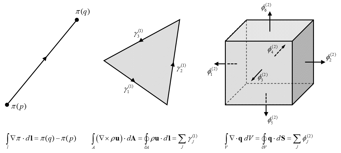
Another view is that the mass flux density is a vector field, denoted \(\mathbf {q}=\rho \mathbf {u}\) where \(\mathbf {u}\) is the flow velocity vector, and the integral of this flux over a cross section \(S\) yields the total amount of mass passing through the cross section in a unit of time. The surface integral is expressed as \[ \int _{S} \mathbf {q}\cdot d\mathbf {S} \] where \(d\mathbf {S}\) is the surface element pointing outward normal to the surface. Here, \(\mathbf {q}\cdot d \mathbf {S}\) represents the mass flux and is physically defined for any size and shape of section \(S\). This physical quantity is another example of a differential form. Note, however, that by Gauss’ divergence theorem in vector calculus, one has \[ \int _V \nabla \cdot \mathbf {q}\,dV = \oint _{\partial V} \mathbf {q}\cdot d\mathbf {S} \] which provides a geometric interpretation of the divergence operator \(\nabla \cdot \) in the sense that integrating this operator over a finite volume yields the total flux through the volume boundaries.
Quantity \(\rho \mathbf {u}\) can also be interpreted as the mass circulation density and is identified with the curl of \(\rho \mathbf {u}\) at a single point: \(\nabla \times \rho \mathbf {u}\). Indeed, by Stokes’ curl theorem, if \(A\) is a finite surface in \(\mathbb {R}^2\) and \(d\mathbf {l}\) is a curve element locally tangent to the boundary of \(A\), then the total circulation of the vector \(\rho \mathbf {u}\) around the perimeter of \(A\) is computed as \[ \oint _{\partial A} \rho \mathbf {u} \cdot d\mathbf {l} = \int _A \left ( \nabla \times \rho \mathbf {u} \right ) \cdot d \mathbf {A} \] Thus, mass circulation is symbolized by the differential form \(\rho \mathbf {u}\cdot d\mathbf {l}\) integrated on a finite line segment.
There are also, however, quantities that can be sampled at single locations, such as surface elevation, bed level and dynamic pressure. These are differential forms associated to a spatial point. Such forms commonly manifest themselves as the argument of the gradient operator \(\nabla \). This is clarified by the fundamental theorem of calculus for line integrals. Let \(\pi : \mathbb {R}^2 \rightarrow \mathbb {R}\) be a differentiable function given on a continuous curve \(\ell \subset \mathbb {R}^2\) that starts at point \(p\) and ends at point \(q\). Then the integral of the gradient of \(\pi \) over the curve \(\ell \) is equal to the total change in \(\pi \) between the two endpoints of \(\ell \), that is, \[ \int _{\ell } \nabla \pi \cdot d\mathbf {l} = \pi (q) - \pi (p) \]
Differential forms are characterized by the dimension of the underlying geometric objects. A differential \(k-\)form integrates over a \(k-\)dimensional smooth (infinitely differentiable) manifold embedded in a \(n-\)dimensional space (\(k=0,1,\dots ,n\)), and takes this to \(\mathbb {R}\). For instance, in \(\mathbb {R}^3\) there are four types of differential forms, that is, \(0-\), \(1-\), \(2-\) and \(3-\)forms, associated with points, curves, planes and volumes, respectively. It is important to note that unlike scalar and vector fields, differential forms are independent of coordinate systems and metric (e.g. length, area, angle).
In what follows, forms are denoted by lower case Greek letters with the superscript indicating the dimension. Hence, with reference to the first example above, \(\mu ^{(3)} = \rho \,dV\) is a \(3-\)form which is a scalar. In the case of the flow velocity vector, there are two distinct differential forms, namely, the \(2-\)form \(\phi ^{(2)} = \mathbf {q}\cdot d\mathbf {S}\), that is, the normal to a plane, and the \(1-\)form \(\gamma ^{(1)} = \rho \mathbf {u}\cdot d\mathbf {l}\), which is the vector tangent to a curve. And in the last example, function \(\pi \) is a \(0-\)form, \(\pi ^{(0)}=\pi \), which trivially gives a scalar.
The calculus of differential forms is based on the exterior derivative and the generalized Stokes’ theorem which extend the notion of differentation and integration, respectively, to arbitrary dimensions. Let \(\mathrm {d}\) denotes the exterior derivative and let \(\alpha ^{(k)}\) be a \(k-\)form defined on some manifold \(\cal M\) of dimension \(k\). The exterior derivative of \(\alpha ^{(k)}\) is a \((k+1)-\)form that is written as \(\mathrm {d}\alpha ^{(k)}\), for \(k = 0, 1, \dots , n-1\). Indeed, the action of exterior derivative on differential forms provides us a coordinate invariant way to calculate the gradient, curl and divergence operators of vector calculus. For example, \(\mathrm {d}\alpha ^{(0)}\) is the same as the gradient of a scalar and the result is a \(1-\)form, which represents a tangential component of a vector. Likewise, \(\mathrm {d}\alpha ^{(1)}\) and \(\mathrm {d}\alpha ^{(2)}\) are equivalent to the curl of a vector (tangent to a curve) and the divergence of a vector (normal to a plane), respectively. The result of the former is a \(2-\)form, which is actually the normal component of a vector, while the result of the latter is scalar, a \(3-\)form.
As we have seen in the above examples, the gradient, curl and divergence operators can be linked to the corresponding geometric objects (curve, plane and volume, respectively) with lower-dimensional boundaries (points, curves and planes, respectively) by means of the corresponding integral theorems (the fundamental theorem of calculus for line integrals, the Stokes’ curl theorem and the Gauss’ divergence theorem, respectively). In the same vein, the exterior derivative can be connected to a \((k+1)-\)dimensional manifold \(\cal M\) with \(k-\)dimensional boundary \(\partial {\cal M}\) through the generalized Stokes’ theorem, which is stated in the following very elegant and simple formula \[ \int _{\cal M} \mathrm {d}\alpha ^{(k)} = \int _{\partial {\cal M}} \alpha ^{(k)} \] for a given \(k-\)form \(\alpha ^{(k)}\). This theorem equates the integral of the exterior derivative of a form on a manifold to the integral of this form on the boundary of the manifold. We observe that the three key theorems of vector calculus as outlined above are all special cases of the generalized Stokes’ theorem.
Differential forms are the essential building blocks in the study of differential geometry [64]. This mathematical language allows one to express differential forms on smooth and curved manifolds in a consistent manner, not dependent on a coordinate system. But most relevant to our discussion is that the use of differential forms is motivated by the physical fact that the measurements of physical quantities, e.g. mass, mass circulation, mass flux, pressure, are typically linked to integration over geometrically finite manifolds. As such, differential forms naturally lend themselves to a discrete representation. In particular, different global variables can be represented as coordinate-free discrete differential forms integrated on different mesh elements (vertices, edges, faces and cells). This is the approach that we will use in the discrete setting.
Consider a three-dimensional computational mesh which consists of vertices, edges, faces and volumes. Let a vertex, an edge, a face and a cell be denoted by \(\sigma _{(k)}\) with \(k = 0, 1, 2, 3\), respectively. A discrete \(k-\)form is defined as the integral of a \(k-\)form over a \(k\)-dimensional mesh element \(\sigma _{(k)}\), symbolized by \[ \int _{\sigma _{(k)}} \alpha ^{(k)} \] and yields a single real number associated with \(\sigma _{(k)}\). Note that the discrete form is the whole integral quantity, not the integrand as with differential forms. In this way, we distinguish between 0-forms represented by their values at a set of vertices, 1-forms by their line integrals over a set of edges, 2-forms by their surface integrals over a set of faces, and 3-forms by their volume integrals over a set of cells. We use from now on Greek letters for discrete forms, that is, \(\pi ^{(0)}\) for the pressure at a vertex, \(\gamma ^{(1)}\) for the mass circulation along a mesh edge, \(\phi ^{(2)}\) for the mass flux through a mesh face, \(\mu ^{(3)}\) for the mass in a cell, etc.
It is also apparent that the discrete forms serve as the degrees of freedom for our numerical framework, rather than grid point values as used in finite difference methods or cell averages in finite volume methods. Since these forms are topological, that is, independent of metric, the intended numerical method can easily be extended to any type of computational meshes embedded in two-dimensional Euclidean spaces, including rectilinear meshes (Chapter 3), curvilinear meshes (Chapter 4) and triangular meshes (Chapter 5).
The generalized Stokes’ theorem reveals that differential forms and integral theorems are intimately connected. More specifically, the integration of a differential form, or the discrete form for that matter, can be used to establish any of the differential operators such as gradient, curl or divergence. This is illustrated by Figure 2.1 that shows the three fundamental theorems with which
the integral of the corresponding differential operator over a finite geometric object is computed by a direct evaluation of the associated discrete form over the boundary of that object. This observation is the central theme for the mimetic discretizations used in this work. In Section 2.5, we will apply the Stokes’ theorem to construct a discrete counterpart of the exterior derivative, with which the continuous differential operators, grad, curl and div can then be mimicked at the discrete level.
In this section we briefly discuss another type of differential form that will not be applied in our discretization process, but utilized as part of the rationale for our choice of associating flow variables with appropriate geometric (mesh) objects. We will come back to this in Section 2.4.5.
With differential \(k-\)forms integrals of scalar and vector fields over a finite \(k-\)dimensional element can be described. Since scalars have no direction and vectors have a single direction, the corresponding differential forms are therefore viewed as a linear map from scalars or vectors to real numbers. Therefore, such differential forms are called a scalar-valued differential form and examples of these include pressure (\(0-\)form), flow velocity (\(1-\)form), mass flux (\(2-\)form), and mass (\(3-\)form).
There are also physical quantities where we need more than one direction to describe their properties. Such quantities typically relate a vector to another vector and are known as tensors. For example, a stress tensor describes fluid deformation normal to a plane but also tangential to the same plane, and is thus a second order tensor with \(n^2\) entries (4 in \(\mathbb {R}^2\) and 9 in \(\mathbb {R}^3\)). In the same way as with scalars and vectors, we can also associate tensors with geometric objects, and they are classified as vector-valued differential forms1 .
To clarify things, we use the conservation of momentum as an example. This fundamental law is expressed by the following Navier-Stokes equation in integral form \[ \frac {\partial }{\partial t} \int _{V} \mathbf {m}\,dV + \oint _{\partial V} \left ( \mathbf {u} \otimes \mathbf {m} - \boldsymbol \tau \right ) \cdot d\mathbf {S} = \int _{V} \mathbf {f} \, dV \] where \(\mathbf {m} = \rho \mathbf {u}\) is the momentum density of the fluid, \(\mathbf {u}\) is is the flow velocity, \(\boldsymbol \tau \) is the (Cauchy) stress tensor and \(\mathbf {f}\) represents body forces acting on the fluid. For Newtonian fluids, the stress tensor reads \[ \boldsymbol \tau = -pI+\mu \left (\nabla \mathbf {u}+(\nabla \mathbf {u})^\mathsf {T} \right ) \] with \(\mu = \rho \nu \) the dynamic viscosity.
Now it is true that convective acceleration, pressure force and viscous stresses in one direction can affect the momentum in another direction. The reason is that momentum density is a vector quantity having both a magnitude and a direction. Yet, not only the amount of momentum is conserved within a control volume, but also in all three spatial directions \(-\) \(x\), \(y\) and \(z\) \(-\) at the same time, viz. \[ \int _{V} \mathbf {m}\,dV \] Here, quantity \(\mathbf {m}\,dV\) is consistently defined for any volume \(V\) and is termed a covector-valued \(3-\)form, that is, it is represented by a scalar-valued \(3-\)form in each physical direction. In the same way, the stress vector \(\boldsymbol \tau \cdot d\mathbf {S}\) is called a covector-valued \(2-\)form (or, generally, \((n-1)-\)form) where each component is associated with plane \(d\mathbf {S}\) with either a normal or a tangential direction. Finally, the convective part of the momentum flux and the body force term are examples of a covector-valued \(2-\)form and a covector-valued \(3-\)form, respectively.
The use of vector-valued differential forms is particularly relevant for the discretization on non-Cartesian meshes. For example, assembling a momentum balance for each component of the momentum density would be rather complicated when the coordinate bases change from point to point so that the momentum flux and stress tensor vary locally both in magnitude and in direction. This requires knowledge on how the covariant (and contravariant) base vectors change spatially which is commonly encoded in the covariant derivative and Christoffel symbols known from tensor calculus [4]. In contrast to scalar-valued differential forms, the mathematical theory of vector-valued differential forms is rather laborious \(-\) this concept is defined without reference to a metric \(-\) and has not received great attention so far in the CFD community. More discussion on this topic is provided in [48].
The present section concludes with a discussion on the associations of the variables in the shallow water equations with suitable geometric elements (points, lines, surfaces, and volumes). These associations are guided by the physical interpretation of the variables. The outline in this section is largely intuitive but will serve as a starting point for a mathematical exposition of the mimetic framework in the sequel of this chapter.
We revisit the inviscid shallow water equations (\(\ref {eq:conteq3}\))\(-\)(\(\ref {eq:momeq3}\)) or (\(\ref {eq:momeq3nc}\)) while examining each variable in the respective equations individually in the following. Recall the continuity equation. It is given by \[ \frac {\partial h}{\partial t} + \nabla \cdot \mathbf {q} = 0 \] The first variable is the water depth \(h\) that acts like a volume and so it is treated as a \(3-\)form. Thereafter, the mass flux \(\mathbf {q}\) is associated with a surface and hence viewed as a \(2-\)form. It should be noted that taking the divergence of a \(2-\)form results in a \(3-\)form. Thus, the continuity equation contains only \(3-\)forms so that the contributions in the equation are mutually consistent.
Next, we continue with the momentum equation which reads \[ \frac {\partial \mathbf {u}}{\partial t} + \left ( \mathbf {u} \cdot \nabla \right ) \, \mathbf {u} = - g \nabla \zeta \] We note here that we are not considering Eq. (\(\ref {eq:momeq3}\)) but rather the equation above. We come back to this point later. The first two terms represent accelerations (temporal and advective, respectively) and are in the same direction as the pressure gradient (Newton’s second law). This direction is tangent to the flow line. Consequently, the advection term \((\mathbf {u} \cdot \nabla ) \, \mathbf {u}\) acts only with one component along this line. This term is thus described as a scalar-valued \(1-\)form. Furthermore, the velocity \(\mathbf {u}\) in the unsteady term measures the fluid flowing along the streamline and is identified as the velocity circulation. (Remember that the projection of \(\mathbf {u}\) onto a line segment \(d\mathbf {l}\), that is \(\mathbf {u}\cdot d\mathbf {l}\), contributes to circulation.) Clearly, this is characterized as a \(1-\)form as well. Finally, the water level \(\zeta \) is sampled at a given location and hence associated with a point. Therefore, it is seen as a \(0-\)form. Since the gradient of a \(0-\)form produces a \(1-\)form, the present equation of motion invariably involves \(1-\)forms only. In this view, Eq. (\(\ref {eq:momeq3nc}\)) will be referred to as the flow equation.
By connecting physical variables to geometric objects more unknowns have been obtained, thus making the system indeterminate. Here, we have four differential forms, symbolically given as \(h\), \(\mathbf {q}\), \(\mathbf {u}\) and \(\zeta \), and two governing equations, implying that two additional relations are required to close the system. In the next section we will see that these so-called constitutive relations are metric dependent and thus approximate in nature. Yet, the distinct use of the differential forms and the constitutive relations allows an elegant way to develop discretizations in a transparent manner by separating the process of approximation from exact discretization. This will be discussed in greater detail in Section 2.6.
As pointed out earlier in this section, the non-conservation form of Eq. (\(\ref {eq:momeq3nc}\)) is utilized to reveal the association between the flow variables and geometry. Let us now turn to the momentum equation (\(\ref {eq:momeq3}\)). The divergence term \(\nabla \cdot \left ( \mathbf {q} \otimes \mathbf {u} \right )\) contains the tensor product between two vectors, viz. \(\otimes \). This implies that Eq. (\(\ref {eq:momeq3}\)) is a tensor equation and thus requires the use of vector-valued differential forms like the Navier-Stokes equations (see the previous section).
Yet, in the context of incompressible shallow water flows, it is assumed that the flow moves gradually downstream as time evolves by which the momentum flux tensor \(\mathbf {q} \otimes \mathbf {u}\) redirects the depth-integrated velocity \(h\mathbf {u}\) towards the direction of the pressure force, with little or no influence from the traversed velocity components. This allows us to stick to Eq. (\(\ref {eq:momeq3nc}\)) while dealing with (vector) differential operators only, such as grad and div, as we did previously. Nevertheless, to handle cases with bores and hydraulic jumps, we will henceforth consider Eq. (\(\ref {eq:momeq3}\)) where all terms are integrated along a streamline, thus treating them as scalar-valued \(1-\)forms. This means that Eq. (\(\ref {eq:momeq3}\)) is interpreted as a flow equation rather than a momentum equation. Note that the time derivative \(\partial h\mathbf {u}/\partial t\) and the pressure gradient term \(g h \nabla \zeta \) are clearly represented by a \(1-\)form since the multiplication of a vector or a gradient (\(1-\)form) by a scalar (\(0-\)form) is still a vector (\(1-\)form).
Another complication concerns the mimetic discretization of momentum advection. In the language of differential forms the treatment of advection is usually by means of the so-called Lie derivative. It expresses the advective transport of a differential form caused by the action of a vector field. Yet, the discretization of the Lie derivative within the mimetic framework is less straightforward. Nevertheless, in their paper [28] the authors showed how for a number of relatively simple cases (e.g. flat domains, regular triangular meshes) there are similarities between the DEC discretizations of the Lie advection of a differential form and the traditional central and upwind schemes within the finite difference and finite volume methods. We will not go into this further, but the interested reader is referred to [23, 62, 48] and [28] for a detailed discussion.
In this work we will use a different approach, proposed by Perot [72] who first developed a staggered mesh discretization of the Navier-Stokes equations in divergence form for unstructured triangular meshes. Accordingly, we will develop a similar discretization for the term \(\nabla \cdot \left ( \mathbf {q} \otimes \mathbf {u} \right )\) separately while adhering to the principles of mimetic discretizations as much as possible. In this regard, this discretization obeys the Rankine-Hugoniot jump relations and thus ensures the correct handling of discontinuities and shocks. A detailed treatment of this approach is described in Chapter 5.
This section concerns with some of the essential definitions and tools of algebraic topology for two-dimensional manifolds. They establish a formalization of the notion of discretization of physical space in which physical laws are embedded. This formalism lay the foundation for the numerical framework of SWASH in the next sections.
Algebraic topology is a branch of mathematics that essentially deals with the study of a manifold (a geometric object) which is encoded by means of the (graph) connectivity. In turn, algebra and discrete boundary relations determined by this connectivity are employed to find topological invariants and symmetries of the manifold implied by differential geometry. As we will see later on, it defines a clean separation between the process of exact discretization of physical conservation properties and the process of approximation of constitutive relations that should be implemented anyway. Original ideas about this approach were proposed two decades ago by [55, 84, 56, 94].
A good introduction to algebraic topology is provided by [63]. Somewhat more abstract is the book of [32]. Another good one on this topic is the (subject to change) lecture notes of [21].
A manifold is a topological space living in \(n-\)dimensional Euclidean space \(\mathbb {R}^n\) that is equipped with a topological structure to allow defining mappings of (sub)manifolds, but not measured by a metric. Such a structure refers to the essential relationships that describe the connectivity between geometric objects and the integral relations that underlie certain invariant and symmetry properties.
A finite dimensional manifold that we will consider here is a computational mesh. It provides a means of partitioning a computational domain \(\Omega \subset \mathbb {R}^n\) into a collection of distinct geometric objects (or submanifolds) called \(k-\)cells with \(k = 0, 1, \dots , n\) indicating their spatial dimension. The associated mesh is thus discretely represented by a finite collection of vertices (\(0-\)cells), edges (\(1-\)cells), faces (\(2-\)cells) and cells (\(3-\)cells).
A \(k-\)cell is denoted by \(\sigma _{(k)}\) and its size or (intrinsic) volume is denoted \(|\sigma _{(k)}|\). We define \(|\sigma _{(0)}|=1\). The collection of \(k-\)cells is a subset of \(\mathbb {R}^n\), denoted \({\cal M}_k\), and is called a \(k-\)dimensional manifold. This manifold is assumed to have a boundary. The boundary of a \(k-\)cell, denoted \(\partial \sigma _{(k)}\), is made up of \((k-1)-\)cells that are directly connected to. These lower dimensional cells are elements of \({\cal M}_{k-1}\) (\(k = 1, \dots , n\)) and are referred to as the faces of the \(k-\)cell. Note that the boundary of a \(0-\)cell is empty. The set \(\{{\cal M}_0,\dots ,{\cal M}_n\}\) is called the mesh.
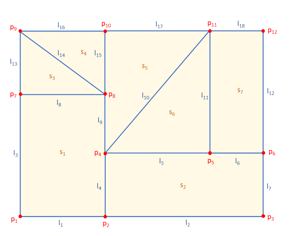
A cell complex \(K\) on \(\Omega \) is a finite set of \(k-\)cells, with \(k = 0, 1, \dots , n\), such that (i) the \(n-\)cells cover \(\Omega \), (ii) each face of a \(k-\)cell of \(K\) is in \(K\), and (iii) the intersection of any two \(k-\)cells of \(K\) is either a face of each of them or is empty. We simply write the cell complex as \(K = \{{\cal M}_0,\dots ,{\cal M}_n\}\), which is a mesh. Note that the converse is not necessarily true (see below). Figure 2.2 illustrates an example of a cell complex in a two-dimensional domain.
Manifolds are also endowed with an orientation which is a key element for identifying the conservation properties in the construction of mimetic discretizations. Two types of orientation can be distinguished for a manifold \({\cal M}_k\): inner and outer orientation. The first type defines the orientation in the geometric object, while the second designates the orientation outside the geometric object embedded in space \(\mathbb {R}^n\).
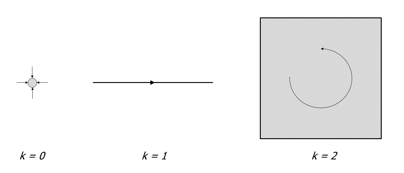
Every \(k-\)cell is oriented and has exactly two directions. In this work, we choose a positive orientation according to the right-hand rule. Consequently, the other is negative. In particular, an inner-oriented \(0-\)cell is positively oriented as a sink (into the vertex), an inner-oriented \(1-\)cell is oriented by a direction, pointing to the right, along the edge, an inner-oriented \(2-\)cell by a sense of rotation, in the counterclockwise direction, on its face and an inner-oriented \(3-\)cell by a right-handed screw inside its cell. Additionally, the inner orientation on \(\partial \sigma _{(k)}\) is induced by \(\sigma _{(k)}\). It is important to note that the inner orientation on a \(k-\)cell is identical for each such cell embedded in an \(n-\)dimensional space.
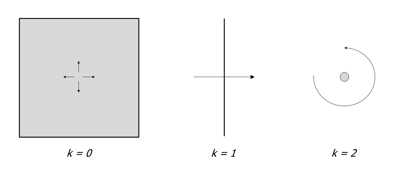
Outer orientation, on the other hand, depends on the dimension of the embedding space. The outer orientation specifies, for instance, a transverse direction through a vertex embedded in \(\mathbb {R}^1\), across an edge in \(\mathbb {R}^2\) and through a face for a 3D embedding space. Here, a positive orientation is the one implied by the orientation of the embedded space that is equipped with a right-handed coordinate system in \(\mathbb {R}^n\). Another example is a counterclockwise rotation around a vertex or an edge embedded in \(\mathbb {R}^2\) and \(\mathbb {R}^3\), respectively. Finally, the outer orientation of an \(n-\)cell in \(\mathbb {R}^n\) is induced by the outer orientation of its faces with outward normals. Thus, the same geometric object has different types of outer orientation depending on the dimension of embedding space \(\mathbb {R}^n\).
The concept of inner and outer orientation gives rise to a pair of meshes embedded in \(\mathbb {R}^n\), each endowed with a different type of orientation. Moreover, they are topologically dual to each other in the sense that an inner-oriented \(k-\)cell corresponds to an outer-oriented \((n-k)-\)cell, and vice versa. The former is referred to as the primal mesh, denoted \(K\), the latter is called the dual mesh, denoted \(\tilde K\). We will use the tilde throughout this chapter to indicate a dual object. Here, \(K\) is inner oriented while \(\tilde K\) is outer oriented, but this is merely a choice and either choice is equally fine. What is important is that all of the \(k-\)cells in one particular mesh must have the same type of orientation (i.e. inner or outer). Figure 2.3 depicts a graphical representation of the orientation of the various primal and dual cells in a 2D space.
The computational mesh is an oriented cell complex \(K\) that covers the domain \(\Omega \). This mesh is designated as the primal mesh. We denote by \(\tilde K\) its associated dual mesh. However, not all faces of the \((n-k)-\)cells in \(\tilde K\) (for \(k = 1, \dots , n\)) are contained in \(\tilde K\). Nevertheless, as we will see later, the dual mesh is not required to be a cell complex in our discretization method. Also, it does not need to be created or stored explicitly \(-\) only its metric will be computed. This will be elaborated in detail in Section 2.5.7.
The topology of the computational mesh is routinely described by means of simplices (e.g. triangles, tetrahedrons) or cuboids (e.g. quadrilaterals, hexahedrons). One should note, however, that both descriptions, though topologically equivalent, are geometrically different; see Section 2.5.7. The present work is entirely devoted to polygonal meshes in \((x,y) \in \Omega \subset \mathbb {R}^2\) even though the space dimension \(n\) is kept general in the present exposition. Here, mesh edges are straight lines and mesh faces are planar. Note that, although there is no difference between the edge and the face of a 2D mesh, their distinction will nevertheless clarify the derivations to be presented.
A polygonal mesh consists of a finite number of polygons. A polygon is said to be cyclic if it can be inscribed in a circle, that is, if there exists a circle so that every vertex of the polygon lies on the circle. This circle is called the circumcircle. For example, all triangles and all rectangles are cyclic. The center of the circumcircle is known as the circumcenter and can be found as the intersection of the perpendicular bisectors of the edges of the polygon.
A polygon is well centered if its circumcenter is contained in its interior. A well-centered computational mesh has all of its polygonal cells that are well centered. For example, an acute triangulation is well centered. The mesh constructed by joining the primal cell circumcenters is called the circumcentric dual mesh. Any well-centered primal mesh and its dual are mutually orthogonal. A classic example is the Delaunay triangulation (primal mesh) and the associated Voronoi tessellation (dual mesh).
Discretizations such as the finite volume and finite element methods benefit from well-centered polygonal meshes because they display desirable conservation and symmetry properties. This is the central theme of this chapter.
Rectangular and curvilinear (cyclic quadrilateral) meshes are always well centered. This is not necessarily true for triangular cells. In particular, the circumcenter of a right-angled triangle lies at the midpoint of the hypotenuse and the circumcenter of an obtuse triangle lies outside the triangle. Nonetheless, one can proof that for every planar polygon there exists a well-centered (nonobtuse) triangulation [5].
An alternative would be the use of the barycentric dual mesh. This mesh is formed by connecting the cell centroids and the edge midpoints. The barycentric dual mesh greatly facilitates flexibility in mesh generation and also in adaptive mesh refinement. However, the lack of orthogonality between the primal edges and their barycentric duals generally increases the complexity of the discretization [35, 57, 58, 59] and may additionally affect the numerical stability.
As will be demonstrated in Section 2.5.7, the circumcentric dual mesh is the preferred one as it allows for computationally tractable and stable discretizations. For the present SWASH applications, only orthogonal rectangular grids (Chapter 3), orthogonal curvilinear grids (Chapter 4) and Delaunay triangular meshes (Chapter 5) are considered.
Let \(C_k(K)\) be a group generated by a basis consisting of all the \(k-\)cells of cell complex \(K\). An element of \(C_k(K)\) is called a \(k-\)chain and is a linear combination of oriented \(k-\)cells, \[ c_{(k)} = \sum _{i} c^i\,\sigma _{(k),i} \] where \(\sigma _{(k),i}\) is the \(i\)th \(k-\)cell in \({\cal M}_k\) and \(c^i \in \{-1,0,1\}\) is the \(i\)th component of \(c_{(k)}\). The \(k-\)cells form the canonical basis for the vector space of \(k-\)chains. The dimension of \(C_k(K)\) equals the number of elements of \({\cal M}_k\) and is written as \(|C_k|\). A \(k-\)chain \(c_{(k)}\) is represented as a row vector of length \(|C_k|\). Furthermore, integer component \(c^i\) of \(c_{(k)}\) refers to the orientation of the cell in the chain with respect to its default orientation in cell complex \(K\) (positive if they agree or negative if they disagree) or to the cell not being a part of the chain, that is, \(c^i = 0\). Note that a \(k-\)cell is also named as an elementary \(k-\)chain.
Just like the boundary of a \(k-\)cell is an element of \({\cal M}_{k-1}\), so is the boundary of a \(k-\)chain, denoted \(\partial c_{(k)}\), an element of \(C_{k-1}(K)\). In this regard, we define the boundary operator as a linear operator \(\partial _k: C_k(K) \rightarrow C_{k-1}(K)\) which returns a \((k-1)-\)chain after applying to the \(k-\)chain, \[ \partial _k c_{(k)} = \partial _k \sum _{i} c^i\,\sigma _{(k),i} \coloneqq \sum _{i} c^i\,\partial _k \sigma _{(k),i} \] with \(\partial _k \sigma _{(k),i}\) the boundary of \(\sigma _{(k),i}\) which is a \((k-1)-\)cell formed by the faces of the oriented \(k-\)cell, as follows \begin {equation} \partial _k \sigma _{(k),i} = \sum _{j} o_{i,j} \, \sigma _{(k-1),j} \label {eq:kcell} \end {equation} where \(o_{i,j}\) equals \(+1\) if \(\sigma _{(k-1),j} \in {\cal M}_{k-1}\) and the orientations of \(\sigma _{(k-1),j}\) and \(\sigma _{(k),i}\) agree, \(-1\) if these orientations disagree, or \(0\) if \(\sigma _{(k-1),j}\) is not a face of \(\sigma _{(k),i}\). Hence, \begin {equation} \partial _k c_{(k)} = \sum _{i} \sum _{j} c^i\,o_{i,j} \, \sigma _{(k-1),j} \label {eq:kchain} \end {equation}
The boundary operator has the important property that the boundary of a boundary is empty, so that using the boundary operator twice to any \(k-\)chain gives a null value, that is, \(\partial _{k-1} \partial _k c_{(k)} = 0\,,\, \forall c_{(k)} \in C_k(K)\). The boundary operator is called nilpotent.
Given a basis for the vector spaces \(C_k(K)\) and \(C_{k-1}(K)\), the boundary operator is represented as an incidence matrix \(\mathbb {D}_k\) of size \(|C_k|\times |C_{k-1}|\). Each row corresponds to each element of \(C_k(K)\) and each column to each element of \(C_{k-1}(K)\). Owing to Eq. (\(\ref {eq:kcell}\)), the entries of the matrix are given by \begin {equation} [\mathbb {D}_k]_{i,j} = o_{i,j}\,,\quad k=1,\dots ,n \label {eq:incmat1} \end {equation} An entry is \(-1\) or \(+1\) (the sign depending on the orientation) if an element of \(C_{k-1}(K)\) is incident with an element of \(C_k(K)\), or 0 if they are not related. Thus the action of boundary operator \(\partial _k\) on a chain \(c_{(k)}\) amounts to the matrix-vector multiplication \(c_{(k)}\,\mathbb {D}_k\), which is a row vector of length \(|C_{k-1}|\). We note that \(c_{(k)}\,\mathbb {D}_k\,\mathbb {D}_{k-1} = \mathbf {0}^\mathsf {T}\,,\, \forall c_{(k)} \in C_{(k)}(K)\,,\, k=2,\dots ,n\).
The vector space of chains \(C_k(K)\) of cell complex \(K\) coexists with a dual vector space of linear functions \(\gamma ^{(k)} \, : \, C_k(K) \rightarrow \mathbb {R}\). This dual space is denoted by \(C^k(K)\) and its elements are called \(k-\)cochains. Let \(c_{(k)}\) be the \(k-\)chain of \(K\) and \(\gamma ^{(k)}\) the \(k-\)cochain of \(K\). We write \[ \langle c_{(k)},\gamma ^{(k)} \rangle \coloneqq \gamma ^{(k)} \,(c_{(k)}\,) \,\, \in \mathbb {R} \] for the value of \(\gamma ^{(k)}\) on \(c_{(k)}\). This linear mapping is called the duality pairing of \(k-\)cochain with \(k-\)chain. As it will be clear shortly, the notion of duality pairing between cochains and chains plays a centrol role in the discretization process.
Given a basis of \(C_k(K)\), \(\{ \sigma _{(k),i} \,| \, i = 1, \dots , |C_k|\}\), there is a dual basis of \(C^k(K)\), \(\{ \sigma ^{(k),i} \, | \, i = 1, \dots , |C_k|\}\), such that \[ \langle \sigma _{(k),j},\sigma ^{(k),i} \rangle = \delta _j^i \] so that the \(i\)th elementary \(k-\)cochain is associated with the \(i\)th \(k-\)cell only. By linearity, a \(k-\)cochain \(\gamma ^{(k)} \in C^k(K)\) can be expressed as \[ \gamma ^{(k)} = \sum _i \gamma _i \sigma ^{(k),i} \] and is represented as a column vector with its components \(\gamma _i \in \mathbb {R}\). The length of this vector is \(|C_k|\). Duality pairing of a \(k-\)cochain \(\gamma ^{(k)}\) with a \(k-\)chain \(c_{(k)}\) can now be calculated as \[ \langle c_{(k)},\gamma ^{(k)} \rangle = \sum _i \sum _j c^j \gamma _i \langle \sigma _{(k),j},\sigma ^{(k),i} \rangle = \sum _i \sum _j c^j \gamma _i \delta _j^i = \sum _i c^i \gamma _i = c_{(k)} \,\gamma ^{(k)} \] This duality pairing is a metric-free operation. (This is not the inner product of Section 2.3 because \(c_{(k)}\) and \(\gamma ^{(k)}\) are not defined in one single vector space.)
A \(k-\)cochain acts as a function that associates to every \(k-\)chain of \(K\) a discrete real number that is independent of any coordinate system. In particular, the value \[ \langle \sigma _{(k),i},\gamma ^{(k)} \rangle = \gamma _i \] is a coordinate-free scalar evaluated on the \(i\)th \(k-\)cell. This function evaluation is interpreted as the geometric integration of \(\gamma ^{(k)}\) over the \(k-\)cell of cell complex \(K\). The integral of \(\gamma ^{(k)}\) over an inner-oriented \(k-\)cell is symbolized by \[ \int _{\sigma _{(k)}} \gamma ^{(k)} \coloneqq \langle \sigma _{(k)},\gamma ^{(k)} \rangle \] and is referred to as an inner-oriented \(k-\)form, or inner \(k-\)form for short. By linearity, the integral of \(\gamma ^{(k)}\) over a \(k-\)chain can be calculated as \[ \int _{c_{(k)}} \gamma ^{(k)} = \sum _i c^i \int _{\sigma _{(k),i}} \gamma ^{(k)} = \sum _i c^i \langle \sigma _{(k),i}, \gamma ^{(k)} \rangle = \sum _i c^i \gamma _i = \langle c_{(k)},\gamma ^{(k)} \rangle \]
Let \(c_{(k+1)}\) be a \((k+1)-\)chain of cell complex \(K\), then its boundary \(\partial _{k+1} c_{(k+1)}\) is a \(k-\)chain. Here, the orientation on \(\partial _{k+1} c_{(k+1)}\) is induced by \(c_{(k+1)}\). The adjoint of this boundary operator with respect to the duality pairing \(\langle \cdot ,\cdot \rangle \) is called the coboundary operator \(\delta ^{k}\) and is defined by \[ \langle c_{(k+1)},\delta ^{k} \gamma ^{(k)} \rangle = \langle \partial _{k+1} c_{(k+1)},\gamma ^{(k)} \rangle \,,\quad \forall c_{(k+1)} \in C_{k+1}(K)\,, \, \forall \gamma ^{(k)} \in C^{k}(K) \] The coboundary operator \(\delta ^k: C^k(K) \rightarrow C^{k+1}(K)\) is a linear operator that relates a \(k-\)cochain to a \((k+1)-\)cochain. The above adjoint relation can also be written in the following integral form \[ \int _{c_{(k+1)}} \delta ^{k} \gamma ^{(k)} = \int _{\partial _{k+1} c_{(k+1)}} \gamma ^{(k)} \] which can be viewed as the discrete counterpart of the generalized Stokes’ theorem. The operator \(\delta ^k\) is also called the \(k\)th discrete exterior derivative. Recall that the three theorems of vector calculus, namely, the fundamental theorem of calculus for line integrals, the Stokes’ curl theorem and the Gauss’ divergence theorem (cf. Figure 2.1) are a special case of the generalized Stokes’ theorem applied to oriented \(0-\)forms, \(1-\)forms and \(2-\)forms, respectively, in \(\mathbb {R}^3\). This observation is key in constructing the mimetic discretization of continuous differential operators grad, curl and div.
The operator \(\delta ^{k}\) can be expressed as an incidence matrix \(\mathbb {D}^k\) of size \(|C_{k+1}|\times |C_k|\) so that the action of \(\mathbb {D}^k\) on a cochain \(\gamma ^{(k)}\) is the matrix-vector multiplication \(\mathbb {D}^k \gamma ^{(k)}\). Matrix \(\mathbb {D}^k\) is the adjoint of matrix \(\mathbb {D}_{k+1}\), which can be demonstrated by the above theorem, namely, \[ c_{(k+1)} \mathbb {D}^k \gamma ^{(k)} = c_{(k+1)} \mathbb {D}_{k+1} \gamma ^{(k)} \] which implies \(\mathbb {D}^k = \mathbb {D}_{k+1}\) for \(k=0,\dots ,n-1\).
By virtue of the duality pairing between the boundary operator and coboundary operator, the discrete exterior derivative is a metric independent operator, which additionally has the property that \[ \mathbb {D}^{k+1}\,\mathbb {D}^k = \mathbf {0}^\mathsf {T}\,,\, \forall k = 0, \dots , n-2 \] reflecting the nilpotency of the coboundary operator, that is, \(\delta ^{(k+1)}\,\delta ^{(k)} = 0\).
Let us choose an inner orientation for cell complex \(K\) in \(\mathbb {R}^2\). Then the discrete exterior derivative represents an exact discretization of grad if \(k=0\) and curl if \(k=1\) such that the Stokes’ theorem holds for the associated inner-oriented \(k-\)cells (cf. left and center panels of Figure 2.1, respectively). In addition, we have that \(\mathbb {D}^1 \mathbb {D}^0 = \mathbf {0}^\mathsf {T}\), which implies curl grad = 0 (the curl of a gradient is zero). Exact representation of this vector calculus identity is crucial for a physics-compatible and stable numerical scheme.
The notions of chains, the boundary operator, discrete forms and the discrete exterior derivative can also be applied on the dual mesh. Let \(K\) be a primal mesh (or cell complex) and \(\tilde K\) the associated dual mesh on \(\Omega \subset \mathbb {R}^2\). Remember that the dual mesh is not a cell complex, but we omit this feature here for simplicity as it does not change the exposition in the following.
There exists a bijective map between the dual mesh elements and the primal ones, namely, each \((n-k)-\)cell of the dual mesh is dual to a primal \(k-\)cell, for \(k = 0, \dots , n\). We denote the dual of \(k-\)cell by \({\tilde \sigma }_{(n-k)}\) and the map by \(\star \), that is, \(\star \sigma _{(k)} = {\tilde \sigma }_{(n-k)}\). The set of dual cells is denoted by \({\tilde {\cal M}}_{n-k}\). The dual mesh is then given by \({\tilde K} = \{{\tilde {\cal M}}_n,\dots ,{\tilde {\cal M}}_0\}\). In line with the choice of primal mesh \(K\) in Section 2.5.2, \(\tilde K\) is outer oriented. Recall that the outer orientation of a dual cell depends on the dimension of the embedded space \(\mathbb {R}^n\).
We denote the vector space of dual \(k-\)chains by \(C_{n-k}(\tilde K)\) and its canonical basis by \(\{ {\tilde \sigma }_{(n-k),i} \,| \, i = 1, \dots , |C_{k}|\}\). Similarly, we have the space of dual \(k-\)cochains, denoted \(C^{n-k}(\tilde K)\), generated by its dual basis \(\{ {\tilde \sigma }^{(n-k),i} \,| \, i = 1, \dots , |C_{k}|\}\). The elements of \(C^{n-k}(\tilde K)\) are the dual discrete forms by which an outer \((n-k)-\)form is dual to an inner \(k-\)form.
The boundary of an outer-oriented cell \({\tilde \sigma }_{(n-k+1)}\) of the dual mesh, with \(k = 1, \dots , n\), constitutes a number of connected faces \({\tilde \sigma }_{(n-k)}\), for which not all of them are in the mesh. By duality, we have the dual boundary operator \({\tilde \partial }_{n-k+1}: C_{n-k+1}(\tilde K) \rightarrow C_{n-k}(\tilde K)\) obtained as follows \[ {\tilde \partial }_{n-k+1} {\tilde \sigma }_{(n-k+1),i} = \sum _{j} {\tilde o}_{i,j} \,{\tilde \sigma }_{(n-k),j}\, , \quad i = 1,\dots ,|C_{k-1}|\,, \,\,\, j = 1,\dots ,|C_k| \] with \({\tilde o}_{i,j}\) indicating the outer orientation of \({\tilde \sigma }_{(n-k)}\) induced by \({\tilde \sigma }_{(n-k+1)}\) (+1 if they agree, \(-1\) if they disagree, and 0 otherwise). This orientation coefficient is related to that on the primal mesh, viz. Eq. (\(\ref {eq:kcell}\)), according to \begin {equation} {\tilde o}_{i,j} = (-1)^k \, o_{j,i}\,, \quad \forall k=1,\dots ,n \label {eq:orkcell} \end {equation} Here the sign coefficient follows from Figure 2.3. In particular, the orientation of the inner-oriented 0\(-\)cell is the opposite of the orientation of the outer-oriented 2\(-\)cell while those of the \(1-\)cells have the same orientation.
The coefficients \({\tilde o}_{i,j}\) constitute an incidence matrix \(\mathbb {\tilde D}_{n-k+1}\) of size \(|C_{k-1}| \times |C_k|\) that represents the dual boundary operator \({\tilde \partial }_{n-k+1}\). Eq. (\(\ref {eq:orkcell}\)) is used to establish the relationship between the primal and dual boundary operators as follows \[ \mathbb {\tilde D}_{n-k+1} = (-1)^{k} \left ( \mathbb {D}_{k} \right )^\mathsf {T}\,,\quad k=1,\dots ,n \] Clearly, on the dual mesh we also have \(\mathbb {\tilde D}_k\,\mathbb {\tilde D}_{k-1} = \mathbf {0}\,,\, \forall k = 2, \dots , n\).
A dual coboundary operator can be defined analogously. The dual coboundary operator \({\tilde \delta }^{n-k-1}: C^{n-k-1}(\tilde K) \rightarrow C^{n-k}(\tilde K)\) is the adjoint of the dual boundary operator \({\tilde \partial }_{n-k}\) based on the generalized Stokes’ theorem \[ \langle {\tilde c}_{(n-k)},{\tilde \delta }^{n-k-1} {\tilde \gamma }^{(n-k-1)} \rangle = \langle {\tilde \partial }_{n-k} {\tilde c}_{(n-k)},{\tilde \gamma }^{(n-k-1)} \rangle \] for all \({\tilde c}_{(n-k)} \in C_{n-k}(\tilde K)\) and \({\tilde \gamma }^{(n-k-1)} \in C^{n-k-1}(\tilde K)\). Note that, by virtue of the duality pairing, the dual cochain \({\tilde \gamma }^{(n-k-1)}\) is an outer form that is integrated over the outer-oriented boundary of \({\tilde c}_{(n-k)}\). The dual coboundary operator is represented by a \(|C_k| \times |C_{k+1}|\) matrix \(\mathbb {\tilde D}^{n-k-1}\) and is given by \[ \mathbb {\tilde D}^{n-k-1} = (-1)^{k+1} \left ( \mathbb {D}^k \right )^\mathsf {T}\,,\quad k=0,\dots ,n-1 \] since \(\mathbb {\tilde D}^{n-k-1} = \mathbb {\tilde D}_{n-k}\) (and \(\mathbb {D}^{k} = \mathbb {D}_{k+1}\)) as per the Stokes’ theorem. Additionally, we have \(\mathbb {\tilde D}^{k+1}\,\mathbb {\tilde D}^k = \mathbf {0}\,,\, \forall k = 0, \dots , n-2\).
By virtue of the Stokes’ theorem, the discrete exterior derivative defined on the dual mesh is the same as the dual coboundary operator. The operator \(\mathbb {\tilde D}^{n-k-1}\) turns an integral over a dual \(k-\)cell into a boundary integral, that is, over the boundary of the dual \(k-\)cell, and maps a discrete outer \((n-k-1)-\)form to a discrete outer \((n-k)-\)form. For example, \(\mathbb {\tilde D}^{n-1}\) acting on the outer \((n-1)-\)form, that is, the flux through a mesh face, yields an outer \(n-\)form (volume form). This is exactly the application of the divergence theorem and operator \(\mathbb {\tilde D}^{n-1}\) is thus identified with the operator div (cf. right panel of Figure 2.1). Furthermore, we observe that \(\mathbb {\tilde D}^{n-1} = -(\mathbb {D}^0)^\mathsf {T}\) which is the discrete version of the antisymmetry relation div = \(-\)grad\(^\mathsf {T}\). As demonstrated in Section 2.3, this property plays a vital role in developing a physically consistent and stable numerical scheme. Since this antisymmetry property is a result of integration by parts, its discrete counterpart is identified as a summation-by-parts rule.
Another form of symmetry is found for \(k=1\), namely \(\mathbb {\tilde D}^{n-2} = \left ( \mathbb {D}^1 \right )^\mathsf {T}\). For \(n=2\) and \(n=3\) this yields \(\mathbb {\tilde D}^0 = \left ( \mathbb {D}^1 \right )^\mathsf {T}\) and \(\mathbb {\tilde D}^1 = \left ( \mathbb {D}^1 \right )^\mathsf {T}\), respectively. This is the discrete representation of curl = curl\(^\mathsf {T}\), meaning that the curl operator is symmetric (aka self-adjoint). Finally, it can be observed that expression \(\mathbb {\tilde D}^1 \mathbb {\tilde D}^0 = \mathbf {0}\) for \(n=2\) or \(\mathbb {\tilde D}^2 \mathbb {\tilde D}^1 = \mathbf {0}\) for \(n=3\) discretely represents the identity div curl = 0 (the divergence of a curl is zero).
The duality between the primal and dual mesh elements suggests that we can define a mapping between a primal \(k-\)form and a dual \((n-k)-\)form. In algebraic topology, this mapping is achieved with the help of the discrete Hodge star operator. This discrete operator will be used later on in the discretization process. While the discrete exterior derivative is uniquely determined by the Stokes’ theorem, there is a great variety of discrete Hodge star operators. In a nutshell, a choice of dual mesh induces a choice of discrete Hodge star.
Given the vector space of discrete \(k-\)forms of primal mesh \(K\) on \(\Omega \subset \mathbb {R}^2\), \(C^k(K)\) and its dual, \(C^{n-k}(\tilde K)\), the \(k\)th discrete Hodge star operator is defined as a linear map \(\mathbb {H}^{k} \, : \, C^k(K) \rightarrow C^{n-k}(\tilde K)\) and is represented as a square matrix of size \(|C_k| \times |C_k|\). The structure of the primal Hodge star matrix \(\mathbb {H}^{k}\) (for \(k=0,\dots ,n\)) depends on the dual mesh. In particular, the metric of the mesh geometry, such as the size and shape of the mesh elements, is the key ingredient of the Hodge star operator.
As will be explained in Section 2.5.8, a required condition for numerical stability is that the discrete Hodge star matrix is positive definite and symmetric. For this reason, we will use the circumcentric dual for the construction of a primal discrete Hodge star matrix. Particularly, the DEC (Discrete Exterior Calculus) approach of [35, 23, 24] is adopted in the current work.
Matrix \(\mathbb {H}^{k}\) maps from a primal \(k-\)form to a dual \((n-k)-\)form. This mapping must be consistent in the sense that both the primal and dual quantities have the same density. For example, for a given velocity vector field in \(\mathbb {R}^3\), a primal 1\(-\)form characterizes the total circulation along the primal edge while a dual 2\(-\)form represents the total flux through to the dual face. To be consistent, the primal 1\(-\)form must be scaled by the size of the edge while the dual 2\(-\)form by the size of the face. Thus we wish to have the following \[ \frac {1}{|\star \sigma _{(k)}|} \int _{\star \sigma _{(k)}} \star \gamma ^{(k)} = \frac {1}{|\sigma _{(k)}|} \int _{\sigma _{(k)}} \gamma ^{(k)} \] where \(\star \sigma _{(k)}\) is the dual of the \(k-\)cell \(\sigma _{(k)}\) and \(\star \gamma ^{(k)}\) is the dual of the \(k-\)form \(\gamma ^{(k)}\). Now any primal cell \(\sigma _{(k)}\) and its circumcentric dual \(\star \sigma _{(k)}\) are mutually orthogonal. This implies that for a particular primal cell and its dual, we have \[ \frac {1}{|{\tilde \sigma }_{(n-k),i}|} \langle {\tilde \sigma }_{(n-k),i},\star \gamma ^{(k)} \rangle = \frac {1}{|\sigma _{(k),i}|} \langle \sigma _{(k),i},\gamma ^{(k)} \rangle \] and so, \[ \frac {\star \gamma _i}{|{\tilde \sigma }_{(n-k),i}|} = \frac {\gamma _i}{|\sigma _{(k),i}|} \] The \(k\)th circumcentric primal Hodge star is thus a diagonal matrix with the entries \[ [\mathbb {H}^{k}]_{i,i} = \frac {|{\tilde \sigma }_{(n-k),i}|}{|\sigma _{(k),i}|}\,,\quad k=0,\dots ,n \] Hence, the action of \(\mathbb {H}^{k}\) on \(\gamma ^{(k)}\) (a column vector) is obtained by the multiplication \(\mathbb {H}^{k} \gamma ^{(k)}\) which is a dual \((n-k)-\)form.
We also define the circumcentric dual Hodge star \(\mathbb {\tilde H}^{n-k}\) which is the map from \(C^{n-k}(\tilde K)\) to \(C^k(K)\), with \(k=0,\dots ,n\), and is simply the inverse of the primal Hodge star, that is, \(\mathbb {\tilde H}^{n-k} = \left (\mathbb {H}^k \right )^{-1}\). This inverse can be found immediately when a circumcentric dual mesh is employed, provided that the primal mesh is well centered. The choice for a circumcentric dual mesh is considered as an advantage compared to a barycentric dual mesh because barycentric primal Hodge matrices are not always invertible while dual Hodge matrices are typically dense due to the loss of the orthogonality property [6]. This advantage will be elaborated in Section 2.5.8.
Let us continue with dimension \(n=2\). As an example, we consider a simplicial mesh consisting of well-centered triangular cells. Figure 2.4 illustrates the different primal and dual \(k-\)cells of a \(2-\)simplex. Their volumes are also indicated in the figure.
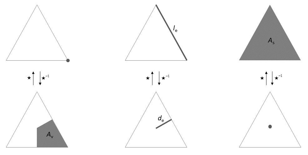
Let \(N_v\), \(N_e\) and \(N_c\) be the number of primal vertices, edges and cells, respectively. The corresponding (circumcentric) primal Hodge star matrices are then given by \begin {equation} [\mathbb {H}^{0}]_{i,i} = A_{\rm v}\,,\quad i=1,\dots ,N_v \label {eq:h0} \end {equation} \begin {equation} [\mathbb {H}^{1}]_{i,i} = \frac {d_{\rm e}}{l_{\rm e}} \,,\quad i=1,\dots ,N_e \label {eq:h1} \end {equation} \begin {equation} [\mathbb {H}^{2}]_{i,i} = \frac {1}{A_{\rm s}}\,,\quad i=1,\dots ,N_c \label {eq:h2} \end {equation} Clearly, the entries of the Hodge matrices are metric dependent and are generally not dimensionless. It is interesting to note that the geometric interpretation of the action of Hodge matrix \(\mathbb {H}^{1}\) is a rotation of a vector in \(\mathbb {R}^2\) counterclockwise by 90\(^o\). In addition, matrix \(\mathbb {H}^{0}\) converts a scalar field to an area-integrated field while the action of \(\mathbb {H}^{2}\) is to get a cell-averaged value of the cell-integrated field variable.
If the computational mesh is well centered, the above matrices are positive definite. However, for a right-angled triangle, matrix \(\mathbb {H}^{1}\) is singular since the length of the edge dual to its hypotenuse is zero. Moreover, the circumcenter of an obtuse triangle is located outside the triangle, implying that \(\mathbb {H}^{1}\) is negative definite. To overcome these unwanted cases, with SWASH the barycenter (or the centroid) is chosen locally instead of the circumcenter; see Section 2.5.10. Note that in case of a Cartesian mesh, the matrices \(\mathbb {H}^{k}\) (\(k=0,1,2\)) are always positive definite.
A special feature of an invertible Hodge star matrix is that it induces a discrete inner product. Let now \(\alpha ^{(k)}\) and \(\beta ^{(k)}\) be the real-valued \(k-\)forms defined on primal mesh \(K\). An inner product of these two forms is defined by \[ \langle \alpha ^{(k)},\beta ^{(k)} \rangle _{\mathbb {H}^{k}} \coloneqq \left ( \alpha ^{(k)} \right )^{\mathsf {T}}\mathbb {H}^{k} \beta ^{(k)} \] This bilinear operator \(\langle \cdot ,\cdot \rangle _{\mathbb {H}^{k}} : C^{k}(K) \times C^{k}(K) \rightarrow \mathbb {R}\) is symmetric and positive definite, provided that \(\mathbb {H}^{k}\) is a symmetric positive definite matrix. Thus for such a matrix, its inverse exists and is symmetric and positive definite as well. Consequently, another discrete inner product can be provided in the following way, \[ \langle {\tilde \alpha }^{(k)},{\tilde \beta }^{(k)} \rangle _{\mathbb {\tilde H}^{k}} = \left ( {\tilde \alpha }^{(k)} \right )^{\mathsf {T}}\mathbb {\tilde H}^{k} {\tilde \beta }^{(k)} = \left ( {\tilde \beta }^{(k)} \right )^{\mathsf {T}}\left (\mathbb {\tilde H}^{k}\right )^{\mathsf {T}} {\tilde \alpha }^{(k)} = \left ( {\tilde \beta }^{(k)} \right )^{\mathsf {T}}\mathbb {\tilde H}^{k} {\tilde \alpha }^{(k)} = \langle {\tilde \beta }^{(k)},{\tilde \alpha }^{(k)} \rangle _{\mathbb {\tilde H}^{k}} \] where \({\tilde \alpha }^{(k)},{\tilde \beta }^{(k)} \in C^{k}(\tilde K)\).
Next, let the following discrete forms be given \[ {\tilde \beta }^{(n-k)} = \mathbb {H}^{k} \beta ^{(k)}\,,\quad {\alpha }^{(k)} = \mathbb {\tilde H}^{n-k} \,{\tilde \alpha }^{(n-k)} \] then we have \[ \langle \alpha ^{(k)},\beta ^{(k)} \rangle _{\mathbb {H}^{k}} = \left ( \alpha ^{(k)} \right )^{\mathsf {T}} {\tilde \beta }^{(n-k)} \] and \[ \langle {\tilde \alpha }^{(n-k)},{\tilde \beta }^{(n-k)} \rangle _{\mathbb {\tilde H}^{n-k}} = \left ( {\tilde \beta }^{(n-k)} \right )^{\mathsf {T}} {\alpha }^{(k)} \] so that \[ \langle {\tilde \alpha }^{(n-k)},{\tilde \beta }^{(n-k)} \rangle _{\mathbb {\tilde H}^{n-k}} = \langle \alpha ^{(k)},\beta ^{(k)} \rangle _{\mathbb {H}^{k}} \] As a matter of notation, inner products of mixed forms can be written as \[ \langle \alpha ^{(k)},{\tilde \beta }^{(n-k)} \rangle _{\mathbb {H}^{k}} = \langle \alpha ^{(k)},\beta ^{(k)} \rangle _{\mathbb {H}^{k}} \] and similarly, \[ \langle {\tilde \alpha }^{(n-k)},\beta ^{(k)} \rangle _{\mathbb {\tilde H}^{n-k}} = \langle {\tilde \alpha }^{(n-k)},{\tilde \beta }^{(n-k)} \rangle _{\mathbb {\tilde H}^{n-k}} \]
An important aspect of inner products is related to the adjoint of linear operators. Recall from functional analysis that every linear operator on a Hilbert space comes with an adjoint operator, and they have a natural relation with respect to inner products. Let \(V^k\) and \(V^{k+1}\) be inner product vector spaces and \(\mathbb {L}^k : V^k \rightarrow V^{k+1}\) be a linear operator. Then this operator induces an adjoint operator \(\left (\mathbb {L}^{k}\right )^\mathsf {T} : V^{k+1} \rightarrow V^k\) in the following way \[ \langle \mathbb {L}^k \alpha ^{(k)}, \beta ^{(k+1)} \rangle _{\mathbb {H}^{k+1}} = \langle \alpha ^{(k)}, \left (\mathbb {L}^k\right )^\mathsf {T} \beta ^{(k+1)} \rangle _{\mathbb {H}^{k}}\,, \quad \forall \alpha ^{(k)} \in V^k\,,\,\,\forall \beta ^{(k+1)} \in V^{k+1} \] with the inner products defined on the respective vector spaces.
Next, let us consider a linear map from \(V^k\) to itself, denoted \(\mathbb {C}^k : V^k \rightarrow V^k\). This operator is called self-adjoint (or symmetric) if \[ \langle \mathbb {C}^k \alpha ^{(k)}, \beta ^{(k)} \rangle _{\mathbb {H}^{k}} = \langle \alpha ^{(k)}, \mathbb {C}^k \beta ^{(k)} \rangle _{\mathbb {H}^{k}}\,, \quad \forall \alpha ^{(k)}\,,\beta ^{(k)} \in V^k \] implying that \[ \left ( \mathbb {C}^k \right )^\mathsf {T} = \mathbb {C}^k \] In addition, the operator is called skew-adjoint (or skew-symmetric) if \[ \langle \mathbb {C}^k \alpha ^{(k)}, \beta ^{(k)} \rangle _{\mathbb {H}^{k}} = -\langle \alpha ^{(k)}, \mathbb {C}^k \beta ^{(k)} \rangle _{\mathbb {H}^{k}}\,, \quad \forall \alpha ^{(k)}\,,\beta ^{(k)} \in V^k \] and hence, \[ \left ( \mathbb {C}^k \right )^\mathsf {T} = -\mathbb {C}^k \] This operator has the special property that \(\langle \alpha ^{(k)}, \mathbb {C}^k \alpha ^{(k)} \rangle _{\mathbb {H}^{k}} = 0\) for all \(\alpha ^{(k)} \in V^k\).
The role of discrete inner products in the discretization process becomes clear by considering the Hamiltonian of the inviscid shallow water equations (see Section 2.3). In particular, for a given discrete \(k-\)form \(\alpha ^{(k)}\), its energy norm \(\langle \alpha ^{(k)},\alpha ^{(k)} \rangle _{\mathbb {H}^{k}}\) is properly defined by the symmetric positive definite Hodge star, making it possible to derive directly an energy conserving (and thus stable) discretization. The above considerations will be useful later on in Section 2.6.
A cochain complex is a sequence of vector spaces and linear operators \((V^k,\mathbb {L}^k)\) such that \(\mathbb {L}^{k+1}\,\mathbb {L}^k=0\). When these spaces refer to the spaces of discrete forms with the same orientation while the linear operator is the discrete exterior derivative, then this cochain complex is called the discrete de Rham complex.
Using the discrete exterior derivative and discrete Hodge star, a diagram can be composed as illustrated in Figure 2.5.
This diagram reflects on how the discretization process works. The lower part of the diagram is the sequence of spaces of inner-oriented discrete forms \(C^k(K)\) connected with \(\mathbb {D}^k\). This sequence is a cochain complex since \(\mathbb {D}^{k+1}\,\mathbb {D}^k=\mathbf {0}\). The upper part of the diagram constitutes a cochain complex of outer-oriented discrete forms \(C^k(\tilde K)\) with the operator \(\mathbb {\tilde D}^k\) that satisfies the property \(\mathbb {\tilde D}^{k+1}\,\mathbb {\tilde D}^k=\mathbf {0}\). These two oriented cochain complexes are dual with respect to each other. Note that we have tacitly assumed that the primal mesh \(K\) is endowed with inner orientation and the dual mesh \(\tilde K\) with outer orientation, but this is rather an arbitrary choice. (In Section 2.6, we will choose this the other way around.) Finally, the primal and dual complexes are connected by the Hodge star operator, which completes the double de Rham complex as shown in Figure 2.5.
In the discrete setting, the horizontal links are encoded by the incidence matrices based on the topological relations of mesh objects. The vertical links are constructed through the Hodge star matrices that are completely metric (or local) dependent. It is precisely this construction that is a determining factor in the development of the numerical framework to be discussed in Section 2.6.
As a first example, the double de Rham complex can be employed to construct the Laplacian of the pressure: \(\Delta p = \nabla \cdot \nabla p\). We start at the bottom left of the diagram by defining an inner \(0-\)form, denoted \(\pi ^{(0)}\). Next, we apply the matrix \(\mathbb {D}^0\) (the gradient) to obtain an inner \(1-\)form. This is followed by the Hodge matrix \(\mathbb {H}^1\) to convert the result to an outer \((n-1)-\)form. (We could have written “\(1-\)form” since \(n=2\), but to emphasize this outer form embedded in \(\mathbb {R}^n\) we use the space dimension.) Then, matrix \(\mathbb {\tilde D}^1\) (the divergence) or \(\mathbb {\tilde D}^{n-1}\) (again to emphasize its relation to outer forms) is applied to get an outer \(n-\)form. Finally, this volume form is transformed back to a point value by means of the Hodge matrix \(\mathbb {\tilde H}^2\) or here \(\mathbb {\tilde H}^n\). (The Laplacian itself is a scalar field function.) Thus, the discretization of the Laplace (or Poisson) operator of the pressure is given by \[ \mathbb {\tilde H}^n\,\mathbb {\tilde D}^{n-1}\,\mathbb {H}^1\,\mathbb {D}^0\,\pi ^{(0)} \] and is considered mimetic because it respects the vector calculus identities and symmetries. This discrete scalar Laplacian can be implemented on arbitrary well-centered meshes, either 2D or 3D, provided that their metric is given.
The second example demonstrates how to discretize \(\Delta \mathbf {u}\). The velocity vector \(\mathbf {u}\) is discretized as an inner \(1-\)form. We denote by \(\upsilon ^{(1)}\) this discrete form. We thus start at the bottom center of the diagram. We can walk through the diagram in two ways. We can first apply the matrix \(\mathbb {D}^1\) (the curl), next the matrix \(\mathbb {H}^2\) followed by \(\mathbb {\tilde D}^{n-2}\) (another curl) and finally matrix \(\mathbb {\tilde H}^{n-1}\). The other route is first \(\mathbb {H}^1\), then \(\mathbb {\tilde D}^{n-1}\) (the divergence), matrix \(\mathbb {\tilde H}^n\) and lastly the matrix \(\mathbb {D}^0\) (the gradient). Now, these two operations together make up the vector Laplacian. Hence, its discretized form reads \[ \mathbb {D}^0 \,\mathbb {\tilde H}^n \,\mathbb {\tilde D}^{n-1} \,\mathbb {H}^1 \,\upsilon ^{(1)} + \mathbb {\tilde H}^{n-1} \,\mathbb {\tilde D}^{n-2} \,\mathbb {H}^2 \,\mathbb {D}^1 \,\upsilon ^{(1)} \] which is precisely the vector calculus identity \(\Delta \mathbf {u} = \nabla \left (\nabla \cdot \mathbf {u}\right ) - \nabla \times \left (\nabla \times \mathbf {u} \right )\). Note, however, that the appearance of the minus sign is enforced because vector calculus does not deal with geometry and orientation.
The above examples demonstrate nicely the strength of the double de Rham complex that provides a natural way to discretize first and second order differential operators while mimicking vector calculus identities. This promotes the physical fidelity and accuracy of the discretization.
In this section we provide some sample calculations to see how things work out in the case of a square cell (or a rectangle), an equilateral triangle cell and a right-angled triangle cell in \(\mathbb {R}^2\) as depicted in Figure 2.6.
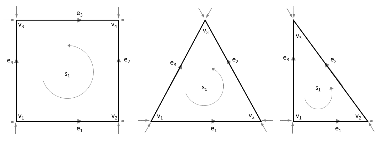
Vertices, edges and the face (either square or triangle) are denoted as \(v_i\), \(e_i\) and \(s_1\), respectively, for \(i= 1,\dots , p\) with \(p=3\) in case of triangles and \(p=4\) in case of the square. The adopted convention for the inner orientation to these mesh elements is shown in the figure, with the condition that the edges are oriented such that they point toward the vertex index of greater value.
Let us consider the square first as shown in Figure 2.6a. This square is a cell complex, denoted \(K_{\rm sq}\). The vertices of this square, \(\{v_1,v_2,v_3,v_4\}\), are the basis of the linear space of \(0-\)chains. Examples of \(0-\)chains are
Similarly, the oriented edges of \(K_{\rm sq}\), \(\{e_1,e_2,e_3,e_4\}\), are the basis of \(C_1(K_{\rm sq})\). A few examples of \(1-\)chains are
The corresponding row vectors are \(\begin {bmatrix} 1 & 0 & 0 & 0 \end {bmatrix}\), \(\begin {bmatrix} 1 & 1 & -1 & 0 \end {bmatrix}\), and \(\begin {bmatrix} -1 & 0 & 0 & 1 \end {bmatrix}\). Next, we can take the boundary of such chains, namely,
Referring to Eq. (\(\ref {eq:kchain}\)), the boundary of the second chain is made up of all \(0-\)chains of cell complex \(K_{\rm sq}\) with coefficients \(c^1 = 1\), \(c^2 = 1\), \(c^3 = -1\), and \(c^4 = 0\), whereas the orientation coefficients are \(o_{1,1} = -1\), \(o_{1,2} = 1\), \(o_{2,1} = -1\), \(o_{2,2} = 1\), \(o_{3,1} = -1\), \(o_{3,2} = 1\), and \(o_{4,1} = -1\), \(o_{4,2} = 1\).
There is only one oriented \(2-\)chain which is \(s_1\). Its boundary equals \[ \partial _2 s_1 = e_1+e_2-e_3-e_4 \] The boundary of this boundary is zero, that is, \[ \partial _1\partial _2 s_1 = \partial _1 e_1 + \partial _1 e_2 - \partial _1 e_3 - \partial _1 e_4 = v_2 - v_1 + v_4 - v_2 + v_3 - v_4 + v_1 - v_3 = 0 \]
By virtue of Eq. (\(\ref {eq:incmat1}\)), the boundary operators \(\partial _1\) and \(\partial _2\) are encoded, respectively, by the following incidence matrices \[ \mathbb {D}_1 = \begin {bmatrix*}[r] -1 & +1 & 0 & 0 \\ 0 & -1 & 0 & +1 \\ 0 & 0 & -1 & +1 \\ -1 & 0 & +1 & 0 \end {bmatrix*} \,,\qquad \mathbb {D}_2 = \begin {bmatrix*}[r] +1 & +1 & -1 & -1 \end {bmatrix*} \] For example, the boundary of the second \(1-\)chain from the above example can be obtained as follows \[ \begin {bmatrix*}[r] 1 & 1 & -1 & 0 \end {bmatrix*} \begin {bmatrix*}[r] -1 & 1 & 0 & 0 \\ 0 & -1 & 0 & 1 \\ 0 & 0 & -1 & 1 \\ -1 & 0 & 1 & 0 \end {bmatrix*} = \begin {bmatrix*}[r] -1 & 0 & 1 & 0 \end {bmatrix*} \] which implies \(\partial _1(e_1+e_2-e_3) = - v_1 + v_3\). One can easily verify that the boundary operator is nilpotent, that is, \(\mathbb {D}_2\,\mathbb {D}_{1} = \mathbf {0}^\mathsf {T}\).
Since the coboundary operator is the dual of the boundary operator, we find \[ \mathbb {D}^0 = \begin {bmatrix*}[r] -1 & +1 & 0 & 0 \\ 0 & -1 & 0 & +1 \\ 0 & 0 & -1 & +1 \\ -1 & 0 & +1 & 0 \end {bmatrix*} \,,\qquad \mathbb {D}^1 = \begin {bmatrix*}[r] +1 & +1 & -1 & -1 \end {bmatrix*} \] Note that these matrices are coordinate independent and hold for an arbitrary (curved) quadrilateral mesh element.
Discrete \(k-\)forms maps an oriented \(k-\)cell to a real value. For instance, a \(0-\)form represents a scalar function that produces its value on vertices. Let us define the pressure \(p\) on vertices \(v_i\), denoted \({\pi }_i = p(v_i)\). This discrete inner \(0-\)form is represented as a column vector with 4 entries. We multiply this vector from the left by matrix \(\mathbb {D}^0\), \[ \begin {bmatrix*}[r] -1 & +1 & 0 & 0 \\ 0 & -1 & 0 & +1 \\ 0 & 0 & -1 & +1 \\ -1 & 0 & +1 & 0 \end {bmatrix*} \begin {bmatrix*}[r] {\pi }_1 \\ {\pi }_2 \\ {\pi }_3 \\ {\pi }_4 \end {bmatrix*} = \begin {bmatrix*} {\pi }_2 - {\pi }_1 \\ {\pi }_4 - {\pi }_2 \\ {\pi }_4 - {\pi }_3 \\ {\pi }_3 - {\pi }_1 \end {bmatrix*} \] This result stems from the generalized Stokes’ theorem, namely, evaluating the exterior derivative of \(p\) on edge \(e_1\) is identical to evaluating \(p\) on the edge boundaries as \(p(v_2) - p(v_1)\). This is simply the classical fundamental theorem of calculus for line integrals. Thus, the value of the \(1-\)form \(\delta ^{(0)}p\) is established as the integral quantity on oriented edges. Matrix \(\mathbb {D}^0\) is therefore the discrete analogue of the gradient operator \(\nabla \).
As a second example, let \({\gamma }_i\) be defined as the circulation along edge \(e_i\). Then operator \(\mathbb {D}^1\) relates this inner \(1-\)form to the inner \(2-\)form, as follows \[ \begin {bmatrix*}[r] +1 & +1 & -1 & -1 \end {bmatrix*} \begin {bmatrix*}[r] {\gamma }_1 \\ {\gamma }_2 \\ {\gamma }_3 \\ {\gamma }_4 \end {bmatrix*} = {\gamma }_1 + {\gamma }_2 - {\gamma }_3 - {\gamma }_4 \] Here, the analogy with the Stokes’ curl theorem is obvious and \(\mathbb {D}^1\) is thus the discrete version of the curl operator \(\nabla \times \). In addition, we find that \(\mathbb {D}^1 \mathbb {D}^0 = \mathbf {0}^\mathsf {T}\), which is the discrete analogue of the identity \(\nabla \times \nabla = \mathbf {0}\).
To summarize, the discrete operators \(\mathbb {D}^0\) and \(\mathbb {D}^1\) represent exactly the continuous gradient and curl operators, respectively, on a 2D primal mesh without reference to any coordinate system.
Next, we turn to the equilateral triangle shown in Figure 2.6b. From this we can deduce the following discrete version of the gradient and the curl, respectively, \[ \mathbb {D}^0 = \begin {bmatrix*}[r] -1 & +1 & 0 \\ 0 & -1 & +1 \\ -1 & 0 & +1 \end {bmatrix*} \,,\quad \mathbb {D}^1 = \begin {bmatrix*}[r] +1 & +1 & -1 \end {bmatrix*} \] Again, we observe that \(\mathbb {D}^1 \mathbb {D}^0 = \mathbf {0}^\mathsf {T}\). Since the boundary and coboundary operators are defined purely topologically, the matrices found above also apply to the right-angled triangle of Figure 2.6c.
In the following, we consider the dual of the square and the triangles as shown in Figure 2.7. The labeling of the mesh elements are now indicated with a tilde.
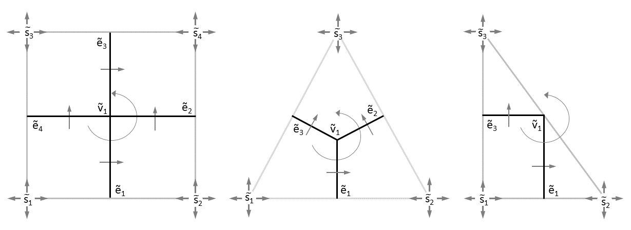
This time we only have one vertex and multiple faces for each mesh cell. Moreover, all the \(1-\)cells and \(2-\)cells are open ended, and therefore the considered mesh cells are not a cell complex. We also notice that one edge is “missing” (its length is zero) in the right triangle cell (Fig. 2.7c).
The outer orientation on the dual cells is depicted in Figure 2.7. For the first example, the dual of the square, the boundary operators acting on dual \(1-\)cells and \(2-\)cells are given by, respectively, \[ {\tilde \partial }_1 \begin {bmatrix*} {\tilde e}_1 \\ {\tilde e}_2 \\ {\tilde e}_3 \\ {\tilde e}_4 \end {bmatrix*} = \begin {bmatrix*}[r] {\tilde v}_1 \\ {\tilde v}_1 \\ -{\tilde v}_1 \\ -{\tilde v}_1 \end {bmatrix*} \,,\qquad {\tilde \partial }_2 \begin {bmatrix*} {\tilde s}_1 \\ {\tilde s}_2 \\ {\tilde s}_3 \\ {\tilde s}_4 \end {bmatrix*} = \begin {bmatrix*}[r] {\tilde e}_1 + {\tilde e}_4 \\ {\tilde e}_2 - {\tilde e}_1 \\ {\tilde e}_3 - {\tilde e}_4 \\ -{\tilde e}_2 - {\tilde e}_3 \end {bmatrix*} \] Subsequently, the coboundary operators can be found as follows \[ \mathbb {\tilde D}^0 = \begin {bmatrix*}[r] +1 \\ +1 \\ -1 \\ -1 \end {bmatrix*} \,,\qquad \mathbb {\tilde D}^1 = \begin {bmatrix*}[r] +1 & 0 & 0 & +1 \\ -1 & +1 & 0 & 0 \\ 0 & 0 & +1 & -1 \\ 0 & -1 & -1 & 0 \end {bmatrix*} \] Note that \(\mathbb {\tilde D}^1\) is the discrete analogue of the divergence operator \(\nabla \cdot \). We also observed that \(\mathbb {\tilde D}^1\) is the negative transpose of \(\mathbb {D}^0\), that is, \(\mathbb {\tilde D}^1 = -(\mathbb {D}^0)^\mathsf {T}\), which is the discrete version of the antisymmetry relation \(\nabla \cdot = -(\nabla )^\mathsf {T}\).
As illustrated by Figure 2.7a, operator \(\mathbb {\tilde D}^0\) is identified with the curl operator. Moreover, we also see that \(\mathbb {\tilde D}^0 = (\mathbb {D}^1)^\mathsf {T}\), which implies \(\nabla \times = (\nabla \times )^\mathsf {T}\). Finally, we find that \(\mathbb {\tilde D}^1 \mathbb {\tilde D}^0 = \mathbf {0}\) which is the discrete representation of \(\nabla \cdot \nabla \times = \mathbf {0}\).
In the same vein, we can derive the coboundary operators for the triangles of Figure 2.7b and 2.7c, which are \[ \mathbb {\tilde D}^0 = \begin {bmatrix*}[r] +1 \\ +1 \\ -1 \end {bmatrix*} \,,\quad \mathbb {\tilde D}^1 = \begin {bmatrix*}[r] +1 & 0 & +1 \\ -1 & +1 & 0 \\ 0 & -1 & -1 \end {bmatrix*} \] Despite the missing edge \({\tilde e}_2\) in the right triangle of Figure 2.7c, one should remember that the coboundary operators are topological, that is, independent of the shape of mesh elements. Finally, one can observe that the above findings related to symmetries and identities remain valid for triangular cells.
Thus far, we have seen that the discrete exterior derivative represents the exact discretization of the differential operators grad, curl, and div in the form of matrices that are purely topological. Such matrices act on coordinate-free variables or physical quantities (discrete forms) defined on vertices, edges and faces. Since the discrete exterior derivative obeys the generalized Stokes’ theorem by construction, the resulting discrete grad, curl, and div operators naturally mimic the vector calculus identities curl grad = 0 and div curl = 0 and the symmetry relations div = \(-\)grad\(^\mathsf {T}\) and curl = curl\(^\mathsf {T}\).
The discrete Hodge star operators, on the contrary, do not depend on the mesh topology, but only on the metric (lengths, areas and volumes) of the various mesh elements. A discrete Hodge star maps between variables living on an inner-oriented mesh and variables living on an outer-oriented mesh. This map always involves some form of approximation. Basically, a choice of discrete Hodge star is much like a choice of dual mesh. Here, we adopted the circumcentric dual like in the examples above (cf. Figure 2.7) which is desired when considering the stability of a numerical scheme.
We now return to the examples to demonstrate how the circumcentric Hodge star matrices are computed. Recall the square of Figure 2.7a. The size of this square is 1 and the circumcenter is \((\frac {1}{2},\frac {1}{2})\). Hence, the intrinsic volume of the primal edges is \(|e_i| = 1\), \(i=1,\dots ,4\), and the primal face is \(|s_1| = 1\). Note that \(|v_i|=1\) by definition. Furthermore, we have for the dual edges and faces inside the square, \(|{\tilde e}_i| = \frac {1}{2}\) and \(|{\tilde s}_i| = \frac {1}{4}\), \(i=1,\dots ,4\). The Hodge star matrix that acts on 0\(-\), 1\(-\) and 2\(-\)forms is then given by, respectively, \[ \mathbb {H}^0 = \frac {1}{4} \begin {bmatrix*}[r] 1 & 0 & 0 & 0 \\ 0 & 1 & 0 & 0 \\ 0 & 0 & 1 & 0 \\ 0 & 0 & 0 & 1 \end {bmatrix*} \,,\quad \mathbb {H}^1 = \frac {1}{2} \begin {bmatrix*}[r] 1 & 0 & 0 & 0 \\ 0 & 1 & 0 & 0 \\ 0 & 0 & 1 & 0 \\ 0 & 0 & 0 & 1 \end {bmatrix*} \,,\quad \mathbb {H}^2 = \begin {bmatrix*}[r] 1 \end {bmatrix*} \] We can conclude that all the three matrices are diagonal and positive definite.
Next, consider the equilateral triangle of Figure 2.7b. Let \(v_1 = (-\frac {1}{2}\sqrt {3},0)\), \(v_2 = (\frac {1}{2}\sqrt {3},0)\) and \(v_3 = (0,\frac {3}{2})\) be vertices of the triangle. The circumcenter is then \((0,\frac {1}{2})\) and the area of the triangle is \(\frac {3}{4}\sqrt {3}\). Furthermore, \(|e_i| = \sqrt {3}\), \(|{\tilde e}_i| = \frac {1}{2}\), \(|s_1| = \frac {3}{4}\sqrt {3}\) and \(|{\tilde s}_i| = \frac {1}{4}\sqrt {3}\), \(i=1,2,3\). The corresponding Hodge star matrices are then given by \[ \mathbb {H}^0 = \frac {\sqrt {3}}{4} \begin {bmatrix*}[r] 1 & 0 & 0 \\ 0 & 1 & 0 \\ 0 & 0 & 1 \end {bmatrix*} \,,\quad \mathbb {H}^1 = \frac {\sqrt {3}}{6} \begin {bmatrix*}[r] 1 & 0 & 0 \\ 0 & 1 & 0 \\ 0 & 0 & 1 \end {bmatrix*} \,,\quad \mathbb {H}^2 = \frac {4\sqrt {3}}{9} \begin {bmatrix*}[r] 1 \end {bmatrix*} \] which are again symmetric positive definite.
For the final example the vertices of the right triangle of Figure 2.7c are \(v_1 = (0,0)\), \(v_2 = (1,0)\) and \(v_3 = (0,1)\). Thus, with \(|s_1| = \frac {1}{2}\), \(|{\tilde s}_1| = \frac {1}{4}\), \(|{\tilde s}_2| = |{\tilde s}_3| = \frac {1}{8}\), we have \[ \mathbb {H}^0 = \frac {1}{8} \begin {bmatrix*}[r] 2 & 0 & 0 \\ 0 & 1 & 0 \\ 0 & 0 & 1 \end {bmatrix*} \,,\quad \mathbb {H}^2 = \begin {bmatrix*}[r] 2 \end {bmatrix*} \] which are positive definite. Now, the triangle is not well centered since the circumcenter \((\frac {1}{2},\frac {1}{2})\) lies exactly on the longest side of the triangle, meaning that \(|{\tilde e}_2| = 0\). This implies that matrix \(\mathbb {H}^1\) is not invertible because it is a singular matrix, namely, \[ \mathbb {H}^1 = \frac {1}{2} \begin {bmatrix*}[r] 1 & 0 & 0 \\ 0 & 0 & 0 \\ 0 & 0 & 1 \end {bmatrix*} \label {eq:singmat} \] In SWASH, this is remedied by choosing the barycenter (the mean of the three vertices) instead. In the current example, this center is \((\frac {1}{3},\frac {1}{3})\). Consequently, \(|e_1| = |e_3| = 1\), \(|e_2| = \sqrt {2}\), \(|{\tilde e}_1| = |{\tilde e}_3| = \frac {\sqrt {5}}{6}\), \(|{\tilde e}_2| = \frac {\sqrt {2}}{6}\) and \(|{\tilde s}_i| = \frac {1}{6}\), \(i=1,2,3\), which yields \[ \mathbb {H}^0 = \frac {1}{6} \begin {bmatrix*}[r] 1 & 0 & 0 \\ 0 & 1 & 0 \\ 0 & 0 & 1 \end {bmatrix*} \,,\quad \mathbb {H}^1 = \frac {1}{6} \begin {bmatrix*}[r] \sqrt {5} & 0 & 0 \\ 0 & 1 & 0 \\ 0 & 0 & \sqrt {5} \end {bmatrix*} \,,\quad \mathbb {H}^2 = \begin {bmatrix*}[r] 2 \end {bmatrix*} \] In particular, the use of this adapted matrix \(\mathbb {H}^1\) gives rise to a locally inconsistent calculation of a dual \(1-\)form from a primal \(1-\)form and vice versa. (This also holds true for matrix \(\mathbb {H}^0\), but as will become apparent, it will not be used in our discretization method; see Section 2.6.) Yet, in practice we see that the impact of the discretization error induced by this local inconsistency is typically very limited. Note that, in this context, generation of well-centered meshes is not strictly required for our discretization method (see also [59]).
Section 2.5 addressed some key ideas that are invaluable for the discretization process, namely, the discrete forms, the generalized Stokes’ theorem, the discrete exterior derivative and the primal-dual meshes. The reason is threefold.
First, unlike vectors, discrete forms are coordinate and metric free and therefore have the same form and properties in all coordinate systems. Since discrete forms are defined by their values at discrete mesh elements, this also highlights their different roles in the spatial discretization (e.g. mass circulation vs mass flux while both representing the velocity vector).
Secondly, the main application of the generalized Stokes’ theorem is to construct the discrete exterior derivative and, in turn, to derive discrete counterparts of the continuous differential operators, viz. grad, curl and div. Like discrete forms, the associated discrete operators are independent of the coordinate system. Moreover, they have an intrinsically discrete nature that allows their exact representation in the numerical framework, including the vector calculus identities curl grad = 0 and div curl = 0.
Finally, the two types of orientation (inner and outer) of the various mesh elements reveal the primal-dual grid structure of the discretization. This naturally induces the layout of staggered grids that lies at the root of the Arakawa C-grid finite difference method. More importantly, the primal-dual framework enables to construct exact discrete expressions for symmetry relations like div = \(-\)grad\(^\mathsf {T}\), which is required to prevent nonlinear computational instability.
The main benefits of obeying identities and symmetry relations at the discrete level include the compatibility with physics and conservation of energy. In particular, mimetic methods possessing these properties are useful when not all scales of nonlinear motion can be resolved without sacrificing physical accuracy, especially when grid refinement or high order discretizations are insufficient. This means that mimetic methods construct physically consistent numerical schemes that lead to high final accuracy, even though they may display low rates of mesh convergence. This approach is an effective way to deal with under-resolved flow problems such as rapidly varied flows and nonlinear wave transformations featuring energy transfer between various wave scales. In addition, mimetic methods have favorable stability properties and do not suffer from spurious modes. Especially, the Arakawa C-grid method is best known for its stability and efficiency and has attracted great attention of various researchers and engineers in the last five decades.
This section is devoted to deriving a general mimetic framework for the numerical solution of the inviscid shallow water equations (\(\ref {eq:conteq3}\)) and (\(\ref {eq:momeq3}\)) on orthogonal meshes by utilizing the concepts of algebraic topology. This derived framework forms the basis for the classical Arakawa C-grid for rectilinear grids in Chapter 3, for curvilinear grids in Chapter 4, and for unstructured triangular meshes in Chapter 5.
Let \(\Omega \subset \mathbb {R}^2\) be a bounded domain on which Eqs. (\(\ref {eq:conteq3}\))\(-\)(\(\ref {eq:momeq3}\)) are given. This domain is discretized by a well-centered polygonal mesh, either triangular or rectangular. Since the mesh is generated by a mesh generator, its boundary edges are aligned with the domain boundaries. Hence, this mesh is a cell complex, and for that reason, it is considered as the primal mesh. On the other hand, its circumcentric dual is not a cell complex because the boundary of dual cells is missing near the domain boundary. Figure 2.8 shows an example of a triangular mesh and its dual.
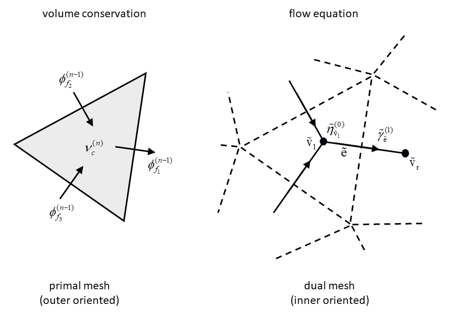
The computational mesh is composed of \(N_v\) vertices, \(N_e\) edges/faces and \(N_c\) cells. Here, we make an explicit distinction between edges as lines (\(1-\)cells) on the one hand, and faces as planes (\((n-1)-\)cells) on the other, even though they are coincident lines in two dimensions (\(n=2\)). It should be noted that the orientation of primal faces induces the orientation of dual edges. Furthermore, by duality, \(N_c\), \(N_e\) and \(N_v\) also give the number of vertices, edges and cells, respectively, in the dual mesh.
We start with the semi-discretization of the continuity equation (\(\ref {eq:conteq3}\)). To enforce mass conservation in every cell of the mesh, we choose the primal mesh to which the discretization of Eq. (\(\ref {eq:conteq3}\)) will be associated. This equation contains two unknowns, namely, \(h\) and \(\mathbf {q}\). The mass flux \(\mathbf {q}\) is encoded by a discrete outer \((n-1)-\)form. It is represented by its surface integrals over the outer-oriented faces of the mesh. Each integral value is constant per planar face. For instance, there are three face values for each primal triangular cell (see left panel of Figure 2.8). Also note that the outer orientation of the face defines a direction of positive flux; see Figure 2.3b. The set of the integral values on faces provides a metric-free representation of the flux field. This set is arranged as a column vector with \(N_e\) entries with each entry assigned to a mesh face. We denote this vector by \(\phi ^{(n-1)}\).
In the context of incompressible shallow water flows with free surface, mass is usually expressed in terms of the volume of the water column, or the water height \(h(\mathbf {x},t)\), while the water density is assumed constant throughout the flow field. Therefore, by mass we refer to the area-integrated height and is treated as an outer discrete \(n-\)form. Its discretization is thus defined on primal \(n-\)cells (here, computational mesh cells). It is an outer-oriented volume form because the net change in the water column is due to the net outflow through the boundaries of the \(n-\)cell (cf. Figure 2.3b). The associated discrete values are stored as elements of a column vector of size \(N_c\), denoted \(\nu ^{(n)}\). (Each entry is given as \(\nu ^{(n)}_c\), see Figure 2.8.)
Clearly, the primal mesh is outer oriented; see left panel of Figure 2.8. Furthermore, when we denote the discrete analogue of the divergence operator by the incidence matrix \(\mathbb {D}^{n-1}\) of size \(N_c \times N_e\), then the semi-discrete version of the continuity equation is given by \begin {equation} \frac {d\nu ^{(n)}}{dt} + \mathbb {D}^{n-1} \phi ^{(n-1)} = 0 \label {eq:dcce} \end {equation} which exactly conserves mass (or volume) in each cell of the mesh. Note that the action of \(\mathbb {D}^{n-1}\) on \(\phi ^{(n-1)}\) results in an \(n-\)form so that Eq. (\(\ref {eq:dcce}\)) consistently contains only outer \(n-\)forms.
By duality, the spatial discretization of the flow equation (\(\ref {eq:momeq3}\)) is implemented on the inner-oriented dual mesh. Starting with the temporal derivative term, the quantity \(h\mathbf {u}\) is discretized as an inner \(1-\)form defined on the dual edges which measures the flow circulation along the cell edges. It is denoted by \({\tilde \gamma }^{(1)}\) which is a column vector of length \(N_e\). Since the dual edges are straight lines, each entry is constant per edge and also defines the flow along the edge (as indicated by \({\tilde \gamma }^{(1)}_{\tilde e}\) in the right panel of Figure 2.8). Accordingly, it describes the flow field on the dual mesh, independent of the coordinate system.
We continue with the right-hand side of Eq. (\(\ref {eq:momeq3}\)) which is the depth-integrated pressure gradient. It represents a driving force along the flow direction. For consistency reasons, the discretization of the term \(h \nabla \zeta \) must be an inner \(1-\)form evaluated on the dual edges. Here, we show how to derive its discretization in a mimetic way.
Let \(\tilde e\) be a dual edge, \({\tilde v}_l\) be its left vertex and \({\tilde v}_r\) its right vertex, see right panel of Figure 2.8. According to the inner orientation of \(1-\)cells (cf. Figure 2.3a), the boundary of \(\tilde e\) is given by \({\tilde \partial }_1 {\tilde e} = {\tilde v}_r - {\tilde v}_l\). Next, let us denote the grid functions (discrete \(0-\)forms) for the free surface, the bed level and the water depth by \(\zeta _i\), \(d_i\) and \(h_i\), respectively, with \(i\) the index of dual vertex \({\tilde v}_i\). By observing that \[ \nabla \, \tfrac {1}{2} g h^2 = g h \nabla \zeta + g h \nabla d \] the application of the dual coboundary operator \({\tilde \delta }^0\) to \(\tfrac {1}{2} g h^2\) on \(\tilde e\) yields \[ \frac {1}{2} g h^2_r - \frac {1}{2} g h^2_l = \frac {1}{2} g \left ( h_r + h_l \right ) \left ( h_r - h_l \right ) = g {\overline h}_{\tilde e} \left ( \zeta _r - \zeta _l \right ) + g {\overline h}_{\tilde e} \left ( d_r - d_l \right ) \] where \({\overline h}_{\tilde e}\) is the arithmetic mean of the two water depths, each on one side of the edge, \[ {\overline h}_{\tilde e} = \frac {1}{2} \left ( h_l + h_r \right ) \] Note that this average value, although associated with the dual edge, is a \(0-\)form. (The sum of two \(k-\)forms is a \(k-\)form.)
The above discretization is exact and provides a discrete expression for the product term \(g h \nabla \zeta \) in terms of inner \(0-\)forms. We first consider both operands separately and then look into the product term.
First, we sample the discrete values of the water depth at the vertices of the dual mesh to form a column vector \({\tilde \eta }^{(0)}\) with \(N_c\) elements (see also right panel of Figure 2.8). We compute the arithmetic mean of this inner \(0-\)form on the dual edges as explained above. We denote this mean by \(\overline {{\tilde \eta }^{(0)}}\). We observe that this action of averaging returns a column vector of length \(N_e\). It is important to note that the arithmetic averaging of an arbitrary discrete form is completely unrelated to the metric.
Next, let us collect all the point values of the water level \(\zeta _i\) into a column vector \({\tilde \zeta }^{(0)}\) of size \(N_c\). The discretization of \(\nabla \zeta \) on the dual mesh is then given by \(\mathbb {\tilde D}^{0} {\tilde \zeta }^{(0)}\) which is the inner \(1-\)form defined on the dual edges. Here, the incidence matrix \(\mathbb {\tilde D}^{0}\) of size \(N_e \times N_c\) represents the discrete gradient operator \({\tilde \delta }^0\) on the dual mesh. Note that by construction \(\mathbb {\tilde D}^{0} = -\left (\mathbb {D}^{n-1}\right )^\mathsf {T}\), which is required to ensure energy conservation (see below). It should also be highlighted that \(\mathbb {\tilde D}^{1}\,\mathbb {\tilde D}^{0} = \mathbf {0}^\mathsf {T}\) which implies that the discrete pressure gradient is curl free. Its practical importance is most evident for rotating flow conditions, as the pressure gradient cannot act as a spurious source of vorticity \(\nabla \times h\mathbf {u}\).
Finally, the mimetic discretization of the pressure gradient \(g h \nabla \zeta \) is given by \[ g \, \overline {{\tilde \eta }^{(0)}} \odot \mathbb {\tilde D}^{0} {\tilde \zeta }^{(0)} \] where \(\odot \) symbolizes the element-wise multiplication of two vectors of the same dimension. This binary operation returns an inner \(1-\)form of the same length. (The multiplication of any \(k-\)form by a \(0-\)form is a \(k-\)form.)
With respect to the second term on the left-hand side of Eq. (\(\ref {eq:momeq3}\)), the conditions imposed on the discretization of the term \(A \mathbf {u} = \nabla \cdot \left ( \mathbf {q} \otimes \mathbf {u} \right )\) are discussed in Section 2.3. In particular, its discretization must result in a matrix with skew-symmetric off-diagonal part, as given by Eq. (\(\ref {eq:mimadv}\)). This will be addressed in detail in Chapters 3, 4 and 5, but for now it is designated as \(\mathbb {A} {\tilde \upsilon }^{(1)}\) which, for consistency, must be an inner \(1-\)form living on dual edges (see also Section 2.4.5). Here, \(\mathbb {A}\) is the discrete version of \(A\) and is encoded as a square matrix of dimension \(N_e \times N_e\). Note that \(\mathbb {A}\) is not a topological operator and is therefore dependent on the metric, which in turn emerges as a principal source of discretization error. Furthermore, we define the inner \(1-\)form \({\tilde \upsilon }^{(1)}\) as the discrete representation of the depth-averaged velocity field \(\mathbf {u}\) integrated along the dual edges. This form is given as a column vector of size \(N_e\).
Putting this all together, the semi-discretization of the flow equation reads \begin {equation} \frac {d {\tilde \gamma }^{(1)}}{dt} + \mathbb {A}{\tilde \upsilon }^{(1)} = -g \, \overline {{\tilde \eta }^{(0)}} \odot \mathbb {\tilde D}^{0} {\tilde \zeta }^{(0)} \label {eq:dcme} \end {equation} The primary unknown here is the cell edge tangential velocity. Consequently, conservation of momentum cannot be guaranteed by this discretization since the full momentum vector is not directly available. (Remember that this would require the use of vector-valued discrete forms.) However, like kinetic energy (see below), the momentum vector field can be reconstructed out of the discrete \(1-\)form and, in turn, a proof of discrete conservation of momentum can then possibly be established.
For example, the \(1-\)form \({\tilde \gamma }^{(1)}\) can be converted into the vector field \(h\mathbf {u}\) by means of the sharp (\(\sharp \)) operator: \(\left ( {\tilde \gamma }^{(1)} \right )^{\sharp } = h\mathbf {u}\) (see, e.g. [48]). Alternatively, given a general coordinate system \(\boldsymbol \xi = (\xi ^1,\xi ^2)\) and the associated unit covariant base vectors \(\mathbf {e}_{(\alpha )} = \mathbf {a}_{(\alpha )} / \sqrt {g_{\alpha \alpha }}\) (no sum) with \(\mathbf {a}_{(\alpha )} = \partial \mathbf {x}/\partial \xi ^\alpha \) and (metric tensor) \(g_{\alpha \alpha } = \mathbf {a}_{(\alpha )} \cdot \mathbf {a}_{(\alpha )}\), the discrete momentum in direction \(\xi ^\alpha \) can be defined as \(\langle \left ( \mathbf {e}_{(\alpha )} \right )^{\flat },{\tilde \gamma }^{(1)}\rangle _{\mathbb {\tilde H}^{1}}\). Here, the flat operator \(\flat \) converts a vector into a \(1-\)form. For an introduction to the operators \(\sharp \) and \(\flat \), also known as the musical isomorphisms, see the lecture notes of [21].
Another example is to derive the discrete momentum vector from the tangential velocity on the cell edges and then subsequently to construct its discrete conservation equation. This is the approach that we will follow in the present work, see Chapter 5.
At this point we observe that Eqs. (\(\ref {eq:dcce}\)) and (\(\ref {eq:dcme}\)), with the exception of the second term \(\mathbb {A}{\tilde \upsilon }^{(1)}\), are exact in the sense that they are independent of the metric. However, there are more unknowns than equations. Five discrete forms can be distinguished of which two are designated as the primary unknowns of the governing equations, namely, the water depth \({\tilde \eta }^{(0)}\) on the dual vertices and the depth-averaged velocity \({\tilde \upsilon }^{(1)}\) on the dual edges. Note that the free surface \({\tilde \zeta }^{(0)}\) can immediately be derived from \({\tilde \eta }^{(0)}\). The other three discrete forms are \(\nu ^{(n)}\), \(\phi ^{(n-1)}\) and \({\tilde \gamma }^{(1)}\).
To close the system of equations it is required to relate these three discrete forms to the prognostic variables. Such relations are commonly called constitutive relations2 and are established by making use of the Hodge star matrices. Note that they require the notion of metric. Based on the de Rham complex diagram of Figure 2.5 we can relate discrete forms defined on the dual mesh to those on the primal mesh, or vice versa, using the Hodge star matrices.
In the following, we will treat the discrete forms \(\phi ^{(n-1)}\), \(\nu ^{(n)}\) and \({\tilde \gamma }^{(1)}\) in turn. First, using the matrix \(\mathbb {\tilde H}^{1}\) we define the constitutive mapping from the depth-averaged velocity circulation along the dual edge (with units of m\(\cdot \)s\(^{-1}\cdot \)m) to the depth-averaged mass flux velocity per unit cross area (given in units of m\(^2\cdot \)s\(^{-1}\cdot \)m\(^{-2}\)) integrated over a primal face (in m\(^2\)) as \[ \upsilon ^{(n-1)} = \mathbb {\tilde H}^{1}\,{\tilde \upsilon }^{(1)} \] Recall that matrix \(\mathbb {\tilde H}^{1}\) is invertible if the computational mesh is well centered. This is thus a critical part of the present method. Next, we define the outer mass flux as \((n-1)-\)form \({\phi }^{(n-1)}\) and it is computed via \(\upsilon ^{(n-1)}\) according to \begin {equation} {\phi }^{(n-1)} = {\upsilon }^{(n-1)} \, \odot \, \overline {{\tilde \eta }^{(0)}} \label {eq:velform} \end {equation} As will become apparent later on, Eq. (\(\ref {eq:velform}\)) is an essential step to achieve discrete energy conservation (see below). This requirement also holds true for nonuniform meshes.
Another discrete constitutive equation takes the following form \[ \nu ^{(n)} = \mathbb {\tilde H}^{0}\,{\tilde \eta }^{(0)} \] with \(\mathbb {\tilde H}^{0}\) relating the water depth (expressed in m) to the volume of the water column (in m\(^3\)). Since this matrix is always invertible (each polygonal cell has non-zero area), we will use its inverse, that is, the primal Hodge matrix \(\mathbb {H}^{n}\).
Since the water depth is one of the variables that is computed explicitly, we wish to express \({\tilde \gamma }^{(1)}\) in terms of a product of \(h\) and \(\mathbf {u}\). To this end, the term \(h\mathbf {u}\) must be considered as a \(1-\)form living on dual edges. Therefore, form \({\tilde \eta }^{(0)}\) must thus be transformed onto edges. This transformation is performed by means of an interpolation matrix of size \(N_e \times N_c\) and the result of this operation is a column vector of length \(N_e\). Note that this operator is a linear map within the dual mesh and thus should not be confused with Hodge star operators.
For the time being, it is not relevant how the interpolation of \({\tilde \eta }^{(0)}\) to dual edges should be done as it is not essential for the explanation of the present framework. Nevertheless, we will see later that certain choices will be made regarding this interpolation and that these are closely related to mass conservation. We will come back to this in Chapters 3, 4 and 5.
As said, form \({\tilde \eta }^{(0)}\) is transformed by averaging onto dual edges and the result is indicated with a tilde, that is, \(\tilde {{\tilde \eta }^{(0)}}\). (The two tildes should not be confused with each other.) This is encoded as a column vector of length \(N_e\). Note that this discrete variable is metric dependent and thus involves some error, which is in contrast with the arithmetic averaging like \(\overline {{\tilde \eta }^{(0)}}\). We now arrive at the expression for \({\tilde \gamma }^{(1)}\) suitable for our framework, namely, \begin {equation} {\tilde \gamma }^{(1)} = \tilde {{\tilde \eta }^{(0)}} \odot {\tilde \upsilon }^{(1)} \label {eq:circform} \end {equation}
With the above discussed approximations, we obtain the following semi-discrete system of equations written in terms of the unknowns \({\tilde \eta }^{(0)}\) and \({\tilde \upsilon }^{(1)}\) \begin {equation} \frac {d{\tilde \eta }^{(0)}}{dt} + \mathbb {H}^{n}\, \mathbb {D}^{n-1} \phi ^{(n-1)} = 0 \label {eq:dcce2} \end {equation} \begin {equation} \frac {d \left ( \tilde {{\tilde \eta }^{(0)}} \odot {\tilde \upsilon }^{(1)} \right )}{dt} + \mathbb {A}{\tilde \upsilon }^{(1)} = -g \, \overline {{\tilde \eta }^{(0)}} \odot \mathbb {\tilde D}^{0} {\tilde \zeta }^{(0)} \label {eq:dcme2} \end {equation} which are ultimately the discretizations of Eqs. (\(\ref {eq:conteq3}\))\(-\)(\(\ref {eq:momeq3}\)). Since the primitive variables live on an inner-oriented dual mesh we call this type of discretizations the inner-oriented discretization. As a side note, we could have chosen an outer-oriented discretization with primitive variables \(\nu ^{(n)}\) and \({\upsilon }^{(n-1)}\), but we have decided not to.
The inner-oriented discretization is essentially a manifestation of the staggered Arakawa C-grid type discretization on orthogonal meshes. Eqs. (\(\ref {eq:dcce2}\))\(-\)(\(\ref {eq:dcme2}\)) represent a suitable basis for the development of the various SWASH discretization methods. As such, it can be applied to simplicial meshes including triangular meshes (see Chapter 5) and to cubical meshes including rectilinear grids (Chapter 3) and curvilinear grids (Chapter 4).
The compatible discretizations of the grad and div operators on primal-dual meshes is key to developing a physically consistent and stable method. With this unique feature, the conservation of the mass and the total energy are satisfied within round-off errors (see below).
As for the discretization of the divergence (or advective) transport term \(\nabla \cdot \left ( \mathbf {q} \otimes \mathbf {u} \right )\), that is, \(\mathbb {A}{\tilde \upsilon }^{(1)}\) in Eq. (\(\ref {eq:dcme2}\)), it is useful to note that it necessarily constitutes a discretization error. Although it is desirable to make this discretization energy conserving, as will be discussed below, there are applications that require some form of dissipation such as, for example, the propagation of bores and wave breaking. The usual approach is to introduce energy dissipation implicitly through the upwind approximation of the divergence term. As demonstrated by e.g. [112, 114], this numerical treatment allows an accurate regularization of the shock waves while stabilizing the semi-discretization. This will be further discussed in Chapters 3, 4 and 5.
Here we proof that the system of equations (\(\ref {eq:dcce2}\))\(-\)(\(\ref {eq:dcme2}\)), or alternatively Eqs. (\(\ref {eq:dcce}\))\(-\)(\(\ref {eq:dcme}\)) is a Hamiltonian system. The discrete version of the total energy of the system is given by \[ {\cal H} = {\cal H}_{\rm kin} + {\cal H}_{\rm pot} = \frac {1}{2} \langle {\upsilon }^{(n-1)},\phi ^{(n-1)} \rangle _{\mathbb {H}^{n-1}} + \frac {1}{2} g \langle {\tilde \zeta }^{(0)},{\tilde \zeta }^{(0)} \rangle _{\mathbb {\tilde H}^{0}} \] and is well defined, provided that the discrete inner products are positive definite and symmetric. We will regularly use the algebraic properties of these inner products as outlined in Section 2.5.8. Let us consider the two contributions of the discrete Hamiltonian separately, first the kinetic energy part and then the potential energy part.
The discrete kinetic energy is defined by \[ \frac {1}{2} \langle {\tilde \upsilon }^{(1)},{\tilde \upsilon }^{(1)}\rangle _{\mathbb {\tilde H}^{1}} = \frac {1}{2} \langle {\upsilon }^{(n-1)},{\tilde \upsilon }^{(1)}\rangle _{\mathbb {H}^{n-1}} \] By analogy with its continuous equivalent, the rate of change of the discrete \({\cal H}_{\rm kin}\) reads \begin {equation} \frac {d{\cal H}_{\rm kin}}{dt} = -\frac {1}{2} \langle {\upsilon }^{(n-1)},{\tilde \upsilon }^{(1)} \odot \frac {d \,\tilde {{\tilde \eta }^{(0)}}}{dt} \rangle _{\mathbb {H}^{n-1}} + \langle {\upsilon }^{(n-1)},\frac {d {\tilde \gamma }^{(1)}}{dt} \rangle _{\mathbb {H}^{n-1}} \label {eq:hkindisc} \end {equation} Note the use of column vector \(\tilde {{\tilde \eta }^{(0)}}\) for expressing the water depth on dual edges. This is consistent with the fact that the kinetic energy part is associated to inner-oriented edges. Here again, the exact definition of this form is not relevant to what follows.
By substituting Eq. (\(\ref {eq:dcme}\)), we obtain the following result \[ \frac {d{\cal H}_{\rm kin}}{dt} = -\frac {1}{2} \langle {\upsilon }^{(n-1)},{\tilde \upsilon }^{(1)} \odot \frac {d \, \tilde {{\tilde \eta }^{(0)}}}{dt} \rangle _{\mathbb {H}^{n-1}} -\langle {\upsilon }^{(n-1)},\mathbb {A} {\tilde \upsilon }^{(1)} \rangle _{\mathbb {H}^{n-1}} -\langle {\upsilon }^{(n-1)},g\,\overline {{\tilde \eta }^{(0)}} \odot \mathbb {\tilde D}^{0} {\tilde \zeta }^{(0)} \rangle _{\mathbb {H}^{n-1}} \] and subsequently using Eq. (\(\ref {eq:velform}\)), we have \begin {equation} \frac {d{\cal H}_{\rm kin}}{dt} = -\frac {1}{2} \langle {\upsilon }^{(n-1)},{\tilde \upsilon }^{(1)} \odot \frac {d \, \tilde {{\tilde \eta }^{(0)}}}{dt} \rangle _{\mathbb {H}^{n-1}} -\langle {\upsilon }^{(n-1)},\mathbb {A} {\tilde \upsilon }^{(1)} \rangle _{\mathbb {H}^{n-1}} -\langle \phi ^{(n-1)},g\,\mathbb {\tilde D}^{0} {\tilde \zeta }^{(0)} \rangle _{\mathbb {H}^{n-1}} \label {eq:dhkin1} \end {equation} Note that the definition of \({\phi }^{(n-1)}\) given by Eq. (\(\ref {eq:velform}\)) is required to arrive at the last term of Eq. (\(\ref {eq:dhkin1}\)).
Next, we aim to expand the second term of the right-hand side of Eq. (\(\ref {eq:dhkin1}\)). Let us denote the off-diagonal part of matrix \(\mathbb {A}\) by \(\mathbb {C}\). We assume a proper discretization of \(\mathbb {A}\) so that matrix \(\mathbb {C}\) is skew-symmetric. Based on Eq. (\(\ref {eq:mimadv}\)) the discretization of the second term is given by \[ \langle {\upsilon }^{(n-1)},\mathbb {A} {\tilde \upsilon }^{(1)} \rangle _{\mathbb {H}^{n-1}} = \frac {1}{2}\langle {\upsilon }^{(n-1)},\mathbb {C} {\tilde \upsilon }^{(1)} \rangle _{\mathbb {H}^{n-1}} - \frac {1}{2}\langle {\upsilon }^{(n-1)},\mathbb {C}^\mathsf {T} {\tilde \upsilon }^{(1)} \rangle _{\mathbb {H}^{n-1}} - \frac {1}{2}\langle {\upsilon }^{(n-1)},\frac {d \,\tilde {{\tilde \eta }^{(0)}}}{dt} \odot {\tilde \upsilon }^{(1)} \rangle _{\mathbb {H}^{n-1}} \] Note that the last term follows directly from Eq. (\(\ref {eq:hkindisc}\)) which explains the irrelevance of the averaging step associated with the tilde (see also Section 2.3). The sum of the first two terms of the right-hand side reduces to \[ \langle {\upsilon }^{(n-1)},\mathbb {C} {\tilde \upsilon }^{(1)} \rangle _{\mathbb {H}^{n-1}} = \langle {\upsilon }^{(n-1)},\mathbb {C} \upsilon ^{(n-1)} \rangle _{\mathbb {H}^{n-1}} = 0 \] by virtue of the skew-symmetry property of \(\mathbb {C}\), so that \[ \langle {\upsilon }^{(n-1)},\mathbb {A} {\tilde \upsilon }^{(1)} \rangle _{\mathbb {H}^{n-1}} = -\frac {1}{2}\langle {\upsilon }^{(n-1)},\frac {d \,\tilde {{\tilde \eta }^{(0)}}}{dt} \odot {\tilde \upsilon }^{(1)} \rangle _{\mathbb {H}^{n-1}} \] Then substitution of this result into Eq. (\(\ref {eq:dhkin1}\)) yields \[ \frac {d{\cal H}_{\rm kin}}{dt} = -\langle \phi ^{(n-1)},g\,\mathbb {\tilde D}^{0} {\tilde \zeta }^{(0)} \rangle _{\mathbb {H}^{n-1}} \]
For the second contribution, the discrete analogue of the rate of change of \({\cal H}_{\rm pot}\) is given by \[ \frac {d{\cal H}_{\rm pot}}{dt} = \langle g{\tilde \zeta }^{(0)},\frac {d\nu ^{(n)}}{dt} \rangle _{\mathbb {\tilde H}^{0}} \overset {\underset {\downarrow }{\mathrm {Eq}.~\ref {eq:dcce}}}{=} -\langle g{\tilde \zeta }^{(0)},\mathbb {D}^{n-1}\phi ^{(n-1)} \rangle _{\mathbb {\tilde H}^{0}} \]
Finally, the rate of change of the discrete Hamiltonian reads
where we have use the fact that the discrete gradient is minus the adjoint of the discrete divergence.
In the context of the discretization of incompressible Navier-Stokes equations, Verstappen and Veldman [102] demonstrated that, in the absence of viscosity, discrete kinetic energy is conserved if two fundamental requirements are fulfilled:
Based on the present analysis we can conclude that these requirements also apply to the discretization of the inviscid shallow water equations. However, for the conservation of discrete potential energy another essential condition must be added here, namely:
The governing two-dimensional, primitive variable equations for the depth-averaged, non-hydrostatic, wind-driven, rotating, free surface flow of an incompressible fluid over a rough bed are given by \begin {equation} \frac {\partial \zeta }{\partial t} + \nabla \cdot \mathbf {q} = 0 \label {eq:conteq4} \end {equation} \begin {equation} \frac {\partial h\mathbf {u}}{\partial t} + \nabla \cdot \left ( \mathbf {q} \otimes \mathbf {u} \right ) + g h \nabla \zeta = -\int _{-d}^{\zeta } \nabla p \, dz +\nabla \cdot \left ( \nu _{\mbox {\tiny h}} \, h \nabla \mathbf {u} \right ) - c_f \| \mathbf {u} \| \mathbf {u} + {\boldsymbol \tau }_w -f \, \mathbf {\hat z} \times h \mathbf {u} \label {eq:momeq4} \end {equation} with \(t\) the time and the coordinate directions \(x\), \(y\) and \(z\) aligning in the east, north, and vertical directions, respectively. In addition, \(\mathbf {\hat z}\) is the unit vector pointing upwards. The gradient operator \(\nabla \) used here operates in two dimensions and reads \[ \nabla = \left ( \frac {\partial }{\partial x}\,,\,\frac {\partial }{\partial y} \right )^\mathsf {T} \]
The bed level \(d(x,y)\) is measured from the reference level \(z=0\) (positive downwards), whereas \(\zeta (x,y,t)\) is the surface elevation with respect to the reference level (positive upwards). The water depth is given by \(h(x,y,t)=\zeta (x,y,t)+d(x,y)\).
Furthermore, \(\mathbf {u}=(u,v)\) is the flow velocity with the depth-averaged components \(u(x,y,t)\) and \(v(x,y,t)\) along the \(x\) and \(y\) coordinates, respectively, \(\mathbf {q} = h \mathbf {u}\) is the mass flux, and \(p(x,y,z,t)\) is the non-hydrostatic pressure (normalised by the water density). Bear in mind the difference between the mass flux \(\mathbf {q}\) and the mass circulation level \(h\mathbf {u}\) in Eq. (\(\ref {eq:momeq4}\)).
Finally, the physical model parameters used here are the horizontal eddy viscosity \(\nu _{\mbox {\tiny h}}(x,y,t)\), the dimensionless bottom friction coefficient \(c_f(x,y,t)\), the wind shear stress at free surface \({\boldsymbol \tau }_w\), the Coriolis parameter \(f = 2 \,\Omega \,sin \, \phi \) with \(\Omega \) the angular speed of Earth’s rotation and \(\phi \) the geographic latitude, and the gravitational acceleration \(g\).
The wind shear stress is parametrized as follows \begin {equation} {\boldsymbol \tau }_w = c_d \, \frac {\rho _{\mbox {\tiny air}}}{\rho } \| {\mathbf {u}}_{10} \| {\mathbf {u}}_{10} \label {eq:wshrpar} \end {equation} where \(c_d\) is the wind drag coefficient, \(\rho _{\mbox {\tiny air}}\) and \(\rho \) are the air and water densities, respectively, and \(\mathbf {u}_{10}\) is the wind speed at 10 m above the free surface.
The shallow water equations (\(\ref {eq:conteq4}\)) and (\(\ref {eq:momeq4}\)) are derived from integrating the mass conservation and the momentum balance over the depth, respectively, whereas the total pressure is decomposed into its hydrostatic and non-hydrostatic components (see, e.g. [15, 27, 118]). In the case of a hydrostatic pressure distribution, i.e. \(p \equiv 0\), these equations can be reformulated as a set of nonlinear hyperbolic equations, and may thus generate discontinuous solutions featuring shock waves [51]. Such solutions can readily be understood as weak solutions in the variational context.
Using Leibniz’ rule, a conservative expression for the gradient of non-hydrostatic pressure is obtained [87] \begin {equation} \int _{-d}^{\zeta } \nabla p \, dz = \frac {1}{2} \nabla \left ( h p_{b} \right ) - p_{b} \nabla d \label {eq:nhydprs} \end {equation} with \(p_b\) the non-hydrostatic pressure at the bed. This pressure is associated with the vertical motion that is governed by the following equation \[ \frac {\partial w_{s}}{\partial t} = \frac {2p_{b}}{h} - \frac {\partial w_{b}}{\partial t} \] where \(w_s\) is the velocity in the \(z-\)direction at the free surface. This equation is derived using the Keller-box method to further improve the dispersive behaviour of the waves [87, 118]. The vertical velocity at the bed \(w_b\) can be found by means of the following kinematic condition \[ w_{b} = -\mathbf {u} \cdot \nabla d \qquad \mbox {at } z = -d \] Finally, the system of equations is complete with the following equation \begin {equation} \nabla \cdot \mathbf {u} + \frac {w_{s} - w_{b}}{h} = 0 \label {eq:locmass3} \end {equation} which ensures conservation of local mass.
This chapter is under preparation.
This chapter presents the development of the discretization method for the shallow water equations on unstructured triangular meshes. The approach to follow is broadly in line with the one suggested by [55, 84, 75] and [94] in which a transparent separation between the processes of exact discretization and approximation is established.
By exact discretization we mean the process of translating a system with an infinite number of degrees of freedom, such as Eqs. (\(\ref {eq:conteq4}\)) and (\(\ref {eq:momeq4}\)), into a finite system of equations and unknowns. This resulting system is exact because no approximations have been introduced yet. However, it is underdetermined and its closure is commonly obtained by the addition of a number of constitutive relations between the different degrees of freedom, which involve some sort of approximation. Both the exact discretization and the process of approximation are addressed separately in detail below.
A key element in the present approach is the primal-dual mesh framework. A classic example is the Delaunay triangulation (primal mesh) and the associated Voronoi tessellation (dual mesh). A successful numerical method that exploits the orthogonality properties of the Delaunay-Voronoi mesh is the covolume discretization of [65, 66, 67, 68] and [29, 16] and later popularized by [72]. Additionally, it has attracted great attention of various researchers and engineers in the last two decades (see, e.g. [27, 90, 45, 41, 42, 33] and [113]).
The covolume method is basically an extension of the Cartesian staggered C-grid technique to orthogonal unstructured triangular and tetrahedral meshes and uses the normal velocity component as the primary unknown. The covolume method typically yields convergence of second order for regular meshes and first order otherwise [66, 72]. Another attractive feature of the covolume discretization is the local and global conservation properties as first shown in [72]. In the context of the incompressible Navier-Stokes equations, this discretization conserves mass exactly, but also (vector) derived quantities such as momentum, kinetic energy and vorticity, both globally and locally [74]. In this sense, the covolume method belongs to the class of mimetic discretization methods.
This chapter presents the discretization method that is similar to the covolume method (see also [113]). The plan of this chapter is as follows. In Section 5.2 the discretization of a physical domain and the main characteristics of the associated computational mesh are described. Section 5.3 discuss the metrics of the mesh which is an essential part of the discretization. In Section 5.4 the exact discretization of the inviscid shallow water equations on orthogonal triangular meshes by using the concepts of algebraic topology is outlined. Section 5.5 deals with various interpolation schemes that are required to close the exact semi-discrete system of equations. Section 5.6 is concerned with providing a detailed summary of the present method. Also, some statements are made about the accuracy of the method. Finally, in Section 5.7 the discrete conservation properties of the present method are demonstrated by considering the discrete equation that conserves mass exactly and the conservation of momentum and (mechanical) energy via certain combinations of the discrete equations.
Let \(\Omega \subset \mathbb {R}^2\) represents a simply connected polygonal domain with regular boundary \(\partial \Omega \). This two-dimensional domain is covered by a mesh defined as a finite collection of non-empty disjoint triangles. Each edge of a triangular cell is either uniquely shared by two adjacent cells or belongs to \(\partial \Omega \).
For each triangle vertex a polygon is constructed that constitutes a partition of \(\Omega \) designated as a dual mesh. The common choices are the circumcentric dual and the barycentric dual [75, 94, 57, 6]. The former dual mesh is constructed by joining the cell circumcenters and the latter is formed by connecting the cell centroids and the edge midpoints. Because of the mutual orthogonality between the primal and dual meshes that allows for stable discretizations, we adopt the circumentric dual in the present method. The motivation for this choice is also discussed in Section 2.5.8. However, a suitable triangular mesh should be well centered, meaning that at least a large proportion of the triangular cells contain their circumcenter, so that inaccurate results can be avoided. An example of a triangle that is not well centered is demonstrated on page ??.
The process of discretization requires the location on the computational mesh where one properly defines the physical variables. This is usually determined by the properties of a nonuniform medium, through which the waves (surface waves, internal waves, etc.) propagate, that affect the local flow conditions, either slowly or rapidly. In particular, the bathymetry can change rapidly, especially in the shallow water regime. As such, the bed level is assumed to be piecewise constant on the mesh cells with the discontinuity at the cell faces. For this reason, the computational mesh is chosen as the primal mesh where its boundary faces are aligned with the domain boundaries and internal faces are aligned with bed discontinuities.
Let indices \(c\), \(f\), \(e\) and \(v\) enumerate cells, faces, edges and vertices, respectively, of the primal (computational) mesh. Those of the dual mesh are indicated by a tilde over the corresponding indices. Furthermore, let \(k\) be the dimension of a mesh element (from a vertex having dimension 0 to a cell having dimension 3). Although there is no difference between the edge and the face of a 2D mesh, their distinction will nevertheless clarify the derivations to be presented below while directly applicable to three dimensions.
There is a bijective map (or duality pairing) between the different mesh elements of primal and dual meshes. The dual of a primal cell \(c\) is the vertex of the dual mesh \(\tilde v\), the dual of a primal face \(f\) is the edge of the dual mesh \(\tilde e\), the dual of a primal edge \(e\) is the face of the dual mesh \(\tilde f\), and the dual of a primal vertex \(v\) is the cell of the dual mesh \(\tilde c\). See Section 2.5.6 for further details. However, only the primal elements \(c\) and \(f\) and their respective duals \(\tilde v\) and \(\tilde e\) suffice for the discretization set out below.
The duality between primal and dual mesh objects requires the use of metrics. We denote \(A_c\) the area of cell \(c\), \(S_f\) the length of face \(f\) (or the face area in 3D), and \(l_e\) the length of edge \(e\). Furthermore, we also use subscripts to indicate the center of gravity (or the centroid) of a mesh element. For example, index \(c\) refers to the primal cell centroid and index \(\tilde e\) to the dual edge midpoint. Note, however, that there is, in general, no correspondence between the centroid of a primal mesh element and that of its dual one. For instance, the centroid of the primal face does not always coincide with the dual edge center and also the primal cell center and the dual vertex position are not always the same. They would be, however, if the triangular mesh is regular or uniform.
For the development of the discretization presented here, the main focus is on the dual edge \(\tilde e\) as depicted in the right panel of Figure 2.8. Between the vertices \({\tilde v}_l\) and \({\tilde v}_r\) of this edge is the intersection with the primal face \(f\). This intersection is the centroid of face \(f\) and is located at position \(\mathbf {x}_f\). Let furthermore \(\mathbf {x}_i\) be the location of \({\tilde v}_i\). Note that \(\mathbf {x}_i\) also refers to the cell circumcenters of the computational mesh. Next, we define the position vector \(\mathbf {r}_{fi}\) from point \(\mathbf {x}_i\) to point \(\mathbf {x}_f\), \[ \mathbf {r}_{fi} = \mathbf {x}_f - \mathbf {x}_i \] and we denote its length by \(l_{fi} = \| \mathbf {r}_{fi} \|\). Owing to the orthogonality, we have \[ \frac {\mathbf {r}_{fl}}{l_{fl}} = - \frac {\mathbf {r}_{fr}}{l_{fr}} = \mathbf {t}_{\tilde e} \] where \(\mathbf {t}_{\tilde e}\) is the unit tangent to edge \(\tilde e\) pointing from \(\mathbf {x}_l\) to \(\mathbf {x}_r\). Note that the length of edge \(\tilde e\) can be computed as \(l_{\tilde e} = l_{fl} + l_{fr}\). We can also regard this length as the distance between the two neighboring cell circumcenters with the face located in between them. Because of the one-to-one correspondence between the dual edges and the primal faces we denote by \({{\Delta } s}_f\) this distance. In addition, with \({{\Delta } s}_{fc}\) we mean the distance from cell face midpoint \(f\) to cell circumcenter \(c\).
To construct discretizations of the differential operators an orientation to the mesh elements must be provided first. The choice of orientation is arbitrary. Let us choose the primal mesh to be outer oriented. With reference to the left panel of Figure 2.8, the right-hand rule is adopted to specify the outer orientation of faces in \(\mathbb {R}^2\), the unit normal to face \(f\), denoted \(\mathbf {n}_f\), is oriented to the right/east or upwards/north. Note that its direction can either be inward or outward with respect to cell \(c\). Since the faces are straight the normal vector is constant. Next, \(\mathbf {n}_{c,f}\) denotes the unit vector pointing out of cell \(c\) and normal to face \(f\). The mutual orientation of the unique normal \(\mathbf {n}_f\) and the outward normal \(\mathbf {n}_{c,f}\) at face \(f\) of cell \(c\) is indicated by \(s_{c,f} = \mathbf {n}_f \cdot \mathbf {n}_{c,f} = \pm 1\). Note that we also have \(\mathbf {n}_f = s_{c,f}\,\mathbf {n}_{c,f}\) and \(\mathbf {n}_{c,f} = s_{c,f}\,\mathbf {n}_f\). Finally, the outer orientation of cell \(c\) is determined by its faces with outward normals.
As was observed in Section 2.4, scalar and vector fields are essentially local functions and thus cannot be associated with a finite region of space. Instead, their integrals over a set of \(k\)-dimensional mesh objects are employed as degrees of freedom known as discrete \(k-\)forms. In what follows, discrete forms are denoted by lower case Greek letters.
On the condition that the water depth \(h(\mathbf {x},t)\) is piecewise continuous on the primal mesh with the discontinuities at the faces and the normal component of mass flux \(\mathbf {q}(\mathbf {x},t)\) is continuous across the faces of the primal mesh, their respective discrete forms are then given by \begin {equation} \nu ^{(n)}_c(t) = \int _c h(\mathbf {x},t)dA \label {eq:pvol1} \end {equation} representing the volume of primal cell \(c\) (dimension \(n\)), and \begin {equation} \phi ^{(n-1)}_f(t) = \int _f \mathbf {q}(\mathbf {x},t) \cdot \mathbf {n}_f \, dS \label {eq:pflx1} \end {equation} defining the integral of the normal component of the mass flux over face \(f\) (dimension \(n-1\)). Note that the mass flux tangent to the primal face can exhibit a discontinuity at the face.
Since the boundary operator acting on cell \(c\) is given by (see Eq. (\(\ref {eq:kcell}\)) and Figure 2.8) \[ \partial _n\, c = f_1 - f_2 - f_3 \] the associated coboundary operator then reads \[ \mathbb {D}^{n-1} = \begin {bmatrix*}[r] +1 & -1 & -1 \end {bmatrix*} \] This incidence matrix locally relates three primal face values to one primal cell value. Note that this matrix only depends on the mesh topology and is thus coordinate invariant. For example, the action of \(\mathbb {D}^{n-1}\) on \(\phi ^{(n-1)} = [\phi ^{(n-1)}_{f_1} \,\, \phi ^{(n-1)}_{f_2} \,\, \phi ^{(n-1)}_{f_3}]^\mathsf {T}\) is given by \[ \mathbb {D}^{n-1} \phi ^{(n-1)} = \phi ^{(n-1)}_{f_1} - \phi ^{(n-1)}_{f_2} - \phi ^{(n-1)}_{f_3} \] which represents the divergence of the mass flux at the discrete level. Hence, continuity of volume in cell \(c\) reads \[ \frac {d \,\nu ^{(n)}_{c}(t)}{dt} = -\phi ^{(n-1)}_{f_1}(t) + \phi ^{(n-1)}_{f_2}(t) + \phi ^{(n-1)}_{f_3}(t) \] or \begin {equation} \frac {d \,\nu ^{(n)}_c}{dt} = -\sum _{f \in \partial c}\,s_{c,f}\,\phi ^{(n-1)}_f \label {eq:ddiv1} \end {equation}
We proceed with the discretization on the dual mesh. This mesh is inner oriented and the orientation of dual edge \(\tilde e\) is depicted in the right panel of Figure 2.8. Furthermore, each dual vertex \({\tilde v}_i\) is oriented as a sink by default, so that \({\tilde \partial }_1 {\tilde e} = {\tilde v}_r - {\tilde v}_l\). Hence, we have \[ \mathbb {\tilde D}^{0} = \begin {bmatrix*}[r] -1 & +1 \end {bmatrix*} \] which locally converts two dual nodal quantities into one dual edge quantity. This coboundary operator is the discrete, coordinate-free implementation of grad. Note here that seemingly the antisymmetry relation \(\mathbb {\tilde D}^{0} = -\left ( \mathbb {D}^{n-1}\right )^\mathsf {T}\) does not hold, but this is only the case when we consider the entire mesh (Recall that the dual mesh is not a cell complex; see also Section 2.6.2).
Next, the following discrete \(0-\)forms defined on an inner-oriented dual mesh are considered in the present method \begin {equation} {\tilde \eta }^{(0)}_{{\tilde v}_i}(t) = h_i(t) \label {eq:pvar1} \end {equation} and \[ {\tilde \zeta }^{(0)}_{{\tilde v}_i}(t) = h_i(t) - d_i = \zeta _i(t) \] representing the water depth and the water level, respectively, at vertex \({\tilde v}_i\). Here, the bed level \(d_i\) is assigned to vertex \(i\) of the dual mesh, which is the circumcenter of the computational cells. In addition, integration of the depth-averaged velocity \(\mathbf {u}\) and the depth-integrated velocity \(h\mathbf {u}\) along edge \(\tilde e\) are given as dual \(1-\)forms, as follows \begin {equation} {\tilde \upsilon }^{(1)}_{\tilde e}(t) = \int _{\tilde e} \mathbf {u}(\mathbf {x},t) \cdot \mathbf {t}_{\tilde e} \, dl \label {eq:pvar2} \end {equation} and \begin {equation} {\tilde \gamma }^{(1)}_{\tilde e}(t) = \int _{\tilde e} h(\mathbf {x},t) \, \mathbf {u}(\mathbf {x},t) \cdot \mathbf {t}_{\tilde e} \, dl \label {eq:gam1} \end {equation} respectively. Note that the sign of \({\tilde \upsilon }^{(1)}_{\tilde e}\), and also of \({\tilde \gamma }^{(1)}_{\tilde e}\), indicates the flow direction.
With the above definitions, we can formulate the analogous expression to the flow equation (\(\ref {eq:dcme}\)) for each dual edge \(\tilde e\), as follows \begin {equation} \frac {d\gamma ^{(1)}_{\tilde e}(t)}{dt} + {\tilde \alpha }^{(1)}_{\tilde e}(t) + g \overline {{\tilde \eta }^{(0)}}_{\tilde e} \left ( {\tilde \zeta }^{(0)}_{{\tilde v}_r}(t) - {\tilde \zeta }^{(0)}_{{\tilde v}_l}(t) \right ) = 0 \label {eq:dmom1} \end {equation} with \[ \overline {{\tilde \eta }^{(0)}}_{\tilde e} = \frac {1}{2} \left ( {\tilde \eta }^{(0)}_{{\tilde v}_l} + {\tilde \eta }^{(0)}_{{\tilde v}_r} \right ) \] Furthermore, \({\tilde \alpha }^{(1)}_{\tilde e}\) represents the line integral of a nonlocal vector \(\mathbf {a}\) that acts as a proxy for \(\nabla \cdot \left ( \mathbf {q} \otimes \mathbf {u} \right )\) and is given by \begin {equation} {\tilde \alpha }^{(1)}_{\tilde e}(t) = \int _{\tilde e} \mathbf {a}(\mathbf {x},t) \cdot \mathbf {t}_{\tilde e} \, dl \label {eq:alpha1} \end {equation} In the perspective of rapidly varied flows, Eq. (\(\ref {eq:dmom1}\)) is conceived as integrating along a path between the upstream and downstream points where a hydraulic jump may form at some location between these two endpoints, depending upon the upstream state [114]. The term \({\tilde \alpha }^{(1)}_{\tilde e}\) plays a key role in this. A mimetic discretization of this term is discussed in the section below.
Right now we have one semi-disrete volume equation in each cell of the primal mesh, Eq. (\(\ref {eq:ddiv1}\)), and one semi-discrete flow equation at each edge of the dual mesh, Eq. (\(\ref {eq:dmom1}\)), but six discrete \(k-\)forms at various locations on these meshes, namely, \(\nu ^{(n)}_c\), \(\phi ^{(n-1)}_f\), \({\tilde \eta }^{(0)}_{{\tilde v}_i}\), \({\tilde \upsilon }^{(1)}_{\tilde e}\), \({\tilde \gamma }^{(1)}_{\tilde e}\) and \({\tilde \alpha }^{(1)}_{\tilde e}\). Closure of this system of equations requires to relate these integral variables to each other and subsequently to evaluate them numerically. These aspects are presented in more detail in the next section.
In this section we describe discrete operators by means of interpolation as they are invoked to complete the system of equations (\(\ref {eq:ddiv1}\)) and (\(\ref {eq:dmom1}\)). These operators require the notion of metric and also introduce a numerical error in the present method. A distinction is made between operators that map one discrete form on the dual mesh to another discrete form on the primal mesh, and operators that perform an interpolation on the dual edge only. The first type of operators is known as discrete Hodge operators and the second type is called the edge-based interpolations. We will treat them separately. Also, the numerical evaluation of discrete forms by quadrature is provided.
Since we have chosen for the inner-oriented scheme, the outer forms need to be replaced by the inner forms. This will be done using the circumcentric dual Hodge (diagonal) matrices. Basically, a dual \(k-\)form given on the dual \(k-\)cell is interpolated on the primal \((n-k)-\)cell to find an approximation of its corresponding primal \((n-k)-\)form. Referring to Sections 2.6.2.0 and 2.5.7 (including Figure 2.4), we have the following maps from the dual vertex to the primal cell \begin {equation} \nu _c^{(n)} = A_c\,{\tilde \eta }^{(0)}_{{\tilde v}_i} \label {eq:dho1} \end {equation} and from the dual edge to the primal face \begin {equation} \upsilon _f^{(n-1)} = \frac {S_f}{l_{\tilde e}}\,{\tilde \upsilon }^{(1)}_{\tilde e} \label {eq:dho2} \end {equation} Both mappings are the result of the circumcentric dual mesh which is constructed by connecting the primal cell circumcenters.
Let us rewrite the transform (\(\ref {eq:dho2}\)) as follows \[ \frac {\upsilon _f^{(n-1)}}{S_f} = \frac {{\tilde \upsilon }^{(1)}_{\tilde e}}{l_{\tilde e}} \] The left-hand side represents the average of the normal flux vector at the center of the primal face \(f\) while the right-hand side describes the average of the tangential velocity vector at the center of the dual edge \(\tilde e\). Both midpoint averaging are second order accurate. Since the circumcentric dual mesh is employed, both these vectors are pointing in the same direction. As a consequence, \({\tilde \upsilon }^{(1)}_{\tilde e}/l_{\tilde e}\) is considered as an interpolated value for \(\upsilon _f^{(n-1)}/S_f\) (or vice versa). In general, the face center and the edge center are not the same so that the dual-edge-to-primal-face interpolation (\(\ref {eq:dho2}\)) is first order accurate. However, when the triangular mesh is regular or uniform, it becomes second order accurate.
In a similar vein, the dual-vertex-to-primal-cell interpolation formula (\(\ref {eq:dho1}\)) is first order accurate in case that the centroid of the primal cell does not coincide with the position of the dual vertex, otherwise it is second order accurate. However, we have assumed that the water depth is constant within the cell implying that the interpolation remains first order accurate.
Since every triangular mesh has a Voronoi dual, implying the presence of cell circumcenters, the circumcentric dual interpolation can in principle always be applied. Yet, it may become inaccurate when the mesh is strongly distorted. In particular, interpolation (\(\ref {eq:dho2}\)) becomes indefinite or incorrect when the circumcenter is not located within the cell itself: \(l_{\tilde e}\) can be zero or negative, respectively. So, in practice, it is desirable (though not necessary) to use a well-centered triangular mesh, such that most of the cell circumcenters are close to the cell centroids.
The primary unknowns (or prognostic variables) of the shallow water equations (\(\ref {eq:conteq3}\)) and (\(\ref {eq:momeq3}\)) are the depth-averaged flow velocity \(\mathbf {u}\) and the water depth \(h\). The discrete unknowns of the present inner-oriented discretization method are defined based on the discrete inner \(k-\)forms. These integral variables can be evaluated numerically by an \(m\)-point Gauss quadrature rule with \(m\) the number of degrees of freedom per mesh element. Since the discretization method is designed as a first order method we will commonly use the midpoint rule (\(m=1\)) to approximate the integrals, with some exceptions.
Let us first consider the depth-averaged circulation velocity on dual edges as given by Eq. (\(\ref {eq:pvar2}\)). This line integral is approximated as \begin {equation} {\tilde \upsilon }^{(1)}_{\tilde e} = \int _{\tilde e} \mathbf {u} \cdot \mathbf {t}_{\tilde e} \, dl = u_{\tilde e} \, l_{\tilde e} \label {eq:pvar2a} \end {equation} where \(u_{\tilde e}\) is the depth-averaged edge-tangential velocity assigned to the center of edge \(\tilde e\) and is designated to be the first prognostic variable of the present method.
On a primal face we have the following \((n-1)-\)form given \[ \upsilon ^{(n-1)}_f = \int _f \mathbf {u} \cdot \mathbf {n}_f \, dS \] which represents the depth-averaged mass flux velocity integrated over face \(f\) (see Section 2.6.2.0). Then employing the midpoint rule to calculate this integral yields \begin {equation} \upsilon ^{(n-1)}_f = u_f\, S_f \label {eq:ups1} \end {equation} with \(u_f\) the depth-averaged face normal velocity at face center \(f\). From Eqs. (\(\ref {eq:dho2}\)) and (\(\ref {eq:pvar2a}\)) it follows that \[ S_f\, u_f = \upsilon _f^{(n-1)} = \frac {S_f}{l_{\tilde e}}\,{\tilde \upsilon }_{\tilde e}^{(1)} = S_f\,u_{\tilde e} \] so that \(u_f = u_{\tilde e}\) which is a first order approximation. Again, when the mesh is regular then the midpoint of the dual edge and the center of the primal face are identical and second order accuracy is obtained by this approximation. In practice, this means that these velocity unknowns can be interchanged without affecting the accuracy of our first order discretization method.
The second prognostic variable used in the discretization method is derived from the water depth located at dual vertices. This inner \(0-\)form is given by Eq. (\(\ref {eq:pvar1}\)). The water depth \(h_i\) is thus located at cell circumcenter \(i\). The present method assumes that the bed level \(d\) is piecewise constant on the mesh cells. We will also apply this assumption to the water depth. This is a first order approximation.
On the other hand, the integral of the water depth over the primal cell, that is, Eq. (\(\ref {eq:pvol1}\)), is approximately evaluated in the following way \begin {equation} \nu ^{(n)}_c = h_c\,A_c \label {eq:pvol2} \end {equation} where \(h_c\) is the cell average water depth at the centroid of cell \(c\). From Eq. (\(\ref {eq:dho1}\)) we have that the indices \(i\) (for circumcenter) and \(c\) (for centroid) for the water depth can be interchanged, that is, \(h_c = h_i\).
Part of the discretization concerns the calculation of the mass flux as given by Eq. (\(\ref {eq:velform}\)) and the mass circulation velocity given by Eq. (\(\ref {eq:circform}\)). They are expressed here as \begin {equation} \phi ^{(n-1)}_f = \upsilon ^{(n-1)}_f \, \, \overline {{\tilde \eta }^{(0)}}_{\tilde e} \label {eq:velform2} \end {equation} in which the mass flux is evaluated over the face \(f\), and \begin {equation} {\tilde \gamma }_{\tilde e}^{(1)} = \tilde {{\tilde \eta }^{(0)}}_{\tilde e} \,\, {\tilde \upsilon }_{\tilde e}^{(1)} \label {eq:circform2} \end {equation} whereby the velocity circulation is computed along the edge \(\tilde e\). (Bear in mind that these are the integral variables.) In both cases an average quantity is involved, namely, \(\overline {{\tilde \eta }^{(0)}}_{\tilde e}\) and \(\tilde {{\tilde \eta }^{(0)}}_{\tilde e}\) while the corresponding interpolations are performed entirely on the dual edge.
Let us start with the arithmetic (or simple) average. It is calculated as a point value in the following manner \begin {equation} \overline {{\tilde \eta }^{(0)}}_{\tilde e} = \frac {1}{2} \left ( {\tilde \eta }^{(0)}_{{\tilde v}_l} + {\tilde \eta }^{(0)}_{{\tilde v}_r} \right ) = \frac {1}{2} \left ( h_l + h_r \right ) = {\overline h}_{\tilde e} \label {eq:haver1} \end {equation} Note that this interpolation is mesh independent as it should be because that is essential for energy conservation, and in turn numerical stability. See Section 2.6.2 for details.
Next, the zero-form \(\tilde {{\tilde \eta }^{(0)}}_{\tilde e}\) embodies the average volume or height that is linked with the mass circulation velocity. It expresses the weighted average of the water depth between two endpoints of the the dual edge \(\tilde e\), namely, \({\tilde v}_l\) and \({\tilde v}_r\). We first approximate the discrete \(1-\)form \({\tilde \gamma }^{(1)}_{\tilde e}\) on the dual edge \(\tilde e\), Eq. (\(\ref {eq:gam1}\)). With reference to Section 5.3, integration is carried out using the endpoint values in the following way [73] \begin {equation} {\tilde \gamma }^{(1)}_{\tilde e} = \int _{\tilde e} h \mathbf {u} \cdot \mathbf {t}_{\tilde e} \, dl \approx h_l \mathbf {u}_l \cdot \mathbf {r}_{fl} - h_r \mathbf {u}_r \cdot \mathbf {r}_{fr} = \left ( l_{fl}\,h_l \, \mathbf {u}_l + l_{fr}\,h_r \, \mathbf {u}_r \right ) \cdot \mathbf {t}_{\tilde e} \label {eq:gam2} \end {equation} resulting in a first order approximation for the depth-integrated velocity. Then we assume that the depth-averaged velocity \(u_{\tilde e}\) is constant along the dual edge so that \(\mathbf {u}_l\cdot \mathbf {t}_{\tilde e} = \mathbf {u}_r \cdot \mathbf {t}_{\tilde e} = u_{\tilde e}\). This first order approximation yields \begin {equation} {\tilde \gamma }^{(1)}_{\tilde e} = \left ( l_{fl}\,h_l + l_{fr}\,h_r \right ) u_{\tilde e} = l_{\tilde e}\,{\tilde h}_f\,u_{\tilde e} \label {eq:gam3} \end {equation} with \({\tilde h}_f\) the weighted average water depth as defined by \[ {\tilde h}_f = \frac {l_{fl}}{l_{\tilde e}}\, h_l + \frac {l_{fr}}{l_{\tilde e}}\, h_r \] Because of Eq. (\(\ref {eq:pvar2a}\)) while comparing Eq. (\(\ref {eq:circform2}\)) to Eq. (\(\ref {eq:gam3}\)), we conclude that \(\tilde {{\tilde \eta }^{(0)}}_{\tilde e} = {\tilde h}_f\). This point value is located at face \(f\). (Remember that this is not necessarily the edge center.) Alternatively, it can be expressed in terms of the distances between face and neighboring cell circumenters, \begin {equation} {\tilde h}_f = \frac {{{\Delta } s}_{fl}}{{{\Delta } s}_f}\, h_l + \frac {{{\Delta } s}_{fr}}{{{\Delta } s}_f}\, h_r \label {eq:haver2a} \end {equation}
What follows is the proof that the above construction of \({\tilde h}_f\) preserves the volume of entire domain \(\Omega \) with variable water height \(h\). Since all the computational cells together form the domain, the total volume is expressed as \[ \sum _{c \in \Omega } A_c\,h_c \]
First, a rhombus is constructed by combining two isosceles triangles on either side of a face. Each of these subtriangles is made up of three vertices, namely, the cell circumcenter and the two endpoints of the face. So, the rhombus has two diagonals of which one is the face \(f\) and the other is the edge \(\tilde e\). Its area is given by \(\frac {1}{2} \,S_f \, l_{\tilde e} = \frac {1}{2} \,S_f \, {{\Delta } s}_f\). Next, we consider a rhombic prism where its bottom (bed) and top (free surface) are rhombuses. Since the heights on each side of the face may not be equal, we insert the average height of this prism at the face which reads \({\tilde h}_f\). Hence, the effective volume of the rhombic prism equals \(\frac {1}{2} \,S_f \,{{\Delta } s}_f\,{\tilde h}_f\).
Next, the volume of water in the entire domain \(\Omega \) is obtained by the sum of nonoverlapping prisms over all the faces, as follows \[ \frac {1}{2} \sum _{f \in \Omega } S_f \,{{\Delta } s}_f\,{\tilde h}_f = \frac {1}{2} \sum _{f \in \Omega } S_f \left ( {{\Delta } s}_{fl}\,h_l + {{\Delta } s}_{fr}\,h_r \right ) = \sum _{c \in \Omega } h_c\, \sum _{f \in \partial c} \frac {1}{2} \, {{\Delta } s}_{fc} \, S_f = \sum _{c \in \Omega } h_c\,A_c \] where the second equality displays the conversion of the sum over the faces into the sum over the cells.
The averaging operator (\(\ref {eq:haver2a}\)) is known as the volume-weighted averaging and is not the usual linear interpolation [30, 98]. On uniform grids it is formally second order accurate and becomes first order on arbitrary meshes. However, in their paper [30] the authors demonstrated that the volume averaging operator is second order accurate on meshes that are sufficiently smooth.
This section presents the construction of a discrete version of the divergence term \(\nabla \cdot \left ( \mathbf {q} \otimes \mathbf {u} \right )\). In particular, we aim to approximate the line integral (\(\ref {eq:alpha1}\)) that contributes to the flow equation (\(\ref {eq:dmom1}\)). In terms of discrete forms, this line integral is represented as a \(1-\)form on the dual edge \(\tilde e\), expressed as \({\tilde \alpha }^{(1)}_{\tilde e}\). The discretization of this nonlinear term on simplicial meshes is not straightforward and usually requires the use of coordinate invariant operators including the Lie derivative. Further discussion on this topic can be found in, e.g. [23, 62, 48] and [28]. Instead, the approach developed by Perot [73, 75, 76] is adopted, which is not based on the formalism of algebraic topology.
Since the momentum flux tensor \(\mathbf {q} \otimes \mathbf {u}\) can be naturally defined at cell faces, the obvious way to compute the divergence term is to integrate it over the cell. We define the vector \(\mathbf {a}_c\) as the average of the divergence term over cell \(c\), \[ \mathbf {a}_c = \frac {1}{A_c} \int _c \nabla \cdot \left ( \mathbf {q} \otimes \mathbf {u} \right ) dA = \frac {1}{A_c} \oint _{\partial c} \left ( \mathbf {q} \cdot \mathbf {n}_{c,f} \right ) \, \mathbf {u} \, dS = \frac {1}{A_c} \sum _{f \in \partial c} \int _f \left ( \mathbf {q} \cdot \mathbf {n}_{c,f} \right ) \, \mathbf {u} \, dS \] Assume that the divergence of the tensor field \(\mathbf {q} \otimes \mathbf {u}\) is constant in a triangular cell so that both the mass flux \(\mathbf {q}\) and the depth-averaged velocity \(\mathbf {u}\) vary linearly within the cell while their normals are constant on cell faces [76]. (Bear in mind that the water depth is cell-wise constant.) Then the integral of the momentum flux over the face can be calculated exactly as follows \[ \int _f \left ( \mathbf {q} \cdot \mathbf {n}_{c,f} \right ) \, \mathbf {u} \, dS = \left ( \mathbf {q}_f \cdot \mathbf {n}_{c,f} \right ) \, \mathbf {u}_f \, S_f = s_{c,f}\,\left ( \mathbf {q}_f \cdot \mathbf {n}_f \right ) \, \mathbf {u}_f \, S_f = s_{c,f} \, \phi ^{(n-1)}_f\,\mathbf {u}_f \] with (see Eq. (\(\ref {eq:pflx1}\))) \begin {equation} \phi ^{(n-1)}_f = \int _f \mathbf {q} \cdot \mathbf {n}_f \, dS = \left ( \mathbf {q}_f \cdot \mathbf {n}_f \right ) S_f \label {eq:phi0} \end {equation} the second order face-integrated mass flux at the face centroid \(f\) and \(\mathbf {u}_f\) the transported flow velocity vector at the center of gravity of face \(f\). Hence, the nonvolumetric advection vector \(\mathbf {a}_c\) at each cell center is approximated as \begin {equation} \mathbf {a}_c = \frac {1}{A_c} \sum _{f \in \partial c} s_{c,f} \, \phi ^{(n-1)}_f \,\mathbf {u}_f \label {eq:advdisc0} \end {equation} and is first order accurate because of the above assumption.
Observe that the cell-based advection vector is constituted by the sum of face fluxes. It turns out, as we will see shortly, that this is required by conservation of momentum. See Section 5.7.2 for further details.
As last step, we continue by evaluating the discrete \(1-\)form \({\tilde \alpha }^{(1)}_{\tilde e}\) on the dual edge \(\tilde e\) with the two neighboring cell circumcenters as endpoints. The corresponding line integral is approximated by utilizing the endpoint values as \begin {equation} {\tilde \alpha }^{(1)}_{\tilde e} = \int _{\tilde e} \mathbf {a} \cdot \mathbf {t}_{\tilde e} \, dl \approx \mathbf {a}_l \cdot \mathbf {r}_{fl} - \mathbf {a}_r \cdot \mathbf {r}_{fr} = \left ( l_{fl}\,\mathbf {a}_l + l_{fr}\,\mathbf {a}_r \right ) \cdot \mathbf {t}_{\tilde e} \label {eq:dalph1} \end {equation} This integration is first order accurate regardless of any mesh. Note the similarity with the volume-weighted average formula (\(\ref {eq:gam2}\)). This completes the construction of the term \(\nabla \cdot \left ( \mathbf {q} \otimes \mathbf {u} \right )\).
Before we conclude this section, we must note that the depth-averaged velocity vector \(\mathbf {u}_f\) in Eq. (\(\ref {eq:advdisc0}\)) still needs to be determined. If we were to calculate this vector at the face centroid itself, we would only need to find its tangential component at the same point. However, the tangent velocity can display a discontinuity at the face. On the other hand, we should be reminded that the off-diagonal part of the discretization matrix of \(\nabla \cdot \left ( \mathbf {q} \otimes \mathbf {u} \right )\) must be skew-symmetric in order to construct discrete energy conservation (for the discussion, see Sections 2.3 and 2.6.2.0 but also Section 5.7.3). For this reason, let us consider two adjacent cells \(l\) and \(r\) sharing the face \(f\). To obtain a skew-symmetric contribution to the advection term we must use the following interpolation \[ {\overline {\mathbf {u}}}_f = \frac {1}{2} \left ( \mathbf {u}_l + \mathbf {u}_r \right ) \] where \(\mathbf {u}_c\) is the depth-averaged velocity vector at cell center \(c\). Like \({\overline h}_{\tilde e}\) (see Eq. (\(\ref {eq:haver1}\))), this metric-independent averaging also turns out to be a necessary condition for energy conservation. We will discuss this further later.
We end this section by presenting the final expression for the advection vector, \begin {equation} \mathbf {a}_c = \frac {1}{A_c} \sum _{f \in \partial c} s_{c,f} \, \phi ^{(n-1)}_f \,{\overline {\mathbf {u}}}_f \label {eq:advdisc1} \end {equation} and by noting that a reconstruction is needed to obtain the cell-based velocity vector \(\mathbf {u}_c\). This is covered in the next section.
Vectors are not a natural ingredient within the framework of algebraic topology. They are, however, required for many purposes like computing the advection operator and the Coriolis force, both involving a velocity vector. This section provides the derivation of a vector reconstruction that approximates the vector field in the cell center by using the face normal components.
A reconstruction of two cell vector components from the face normals is always possible as long as each 2D computational cell has at least two nonparallel faces. However, it is not unique. Various reconstruction methods can be found in the literature of which the common ones are the least squares reconstruction of vector fields [67, 80, 103, 71], Whitney forms [107, 11] and the method of Perot using Gauss’ divergence theorem [72, 76].
Least squares approximations typically reconstruct the cell-based vector through the polynomial interpolation from the vector components at the surrounding cell faces. Though these algorithms provide full control over the accuracy of their reconstructions, they are rather involved and computationally demanded [71].
Whitney forms are widely used in computational electromagnetism and can also be applied to construct Hodge star matrices on simplicial meshes [57].
The interpolation method of Perot is a rather intuitive approach and makes no reference to algebraic topology. However, as we will see later, this method is mimetic in the sense that it conserves local kinetic energy (see Section 5.7.3). Another advantage is that it can be applied to arbitrary polygons. For these reasons, we adopt the interpolation method as described in [76].
The starting point is an arbitrary two-dimensional vector field \(\mathbf {u}\) and a 2DH mesh with polygonal cells that are all cyclic (e.g. triangular, rectangles). Furthermore, the projection of this vector on the directions normal to a cell face \(f\) is specified, that is, \(\mathbf {u}_f\cdot \mathbf {n}_{f} = u_f\). (Recall that the normal vector components are well defined on the polygonal faces.) The aim is to reconstruct a cell-centered vector \(\mathbf {u}_c\) out of the face normals \(u_f\).
We do this first by considering the volume integral of the divergence of the tensor field \(\mathbf {u} \otimes \mathbf {r}\) over a cell and subsequently applying the divergence theorem, \[ \int _c \nabla \cdot \left ( \mathbf {u} \otimes \mathbf {r} \right ) dA = \oint _{\partial c} \left ( \mathbf {u} \cdot \mathbf {n}_{c,f} \right ) \, \mathbf {r} \, dS = \sum _{f \in \partial c} \int _f \left ( \mathbf {u} \cdot \mathbf {n}_{c,f} \right ) \, \mathbf {r} \, dS \] where \(\mathbf {r} = \mathbf {x} - \mathbf {x}_c\) is the position vector. The position \(\mathbf {x}_c\) might be the center of gravity or the circumcenter. Expanding the first term, we have \[ \int _c \mathbf {r}\left ( \nabla \cdot \mathbf {u} \right ) dA + \int _c \left ( \mathbf {u} \cdot \nabla \right ) \mathbf {r} dA = \sum _{f \in \partial c} \int _f \left ( \mathbf {u} \cdot \mathbf {n}_{c,f} \right ) \, \mathbf {r} \, dS \]
Next, we assume that vector \(\mathbf {u}\) is constant over cell \(c\), so that \(\nabla \cdot \mathbf {u}= 0\). By observing that \(\left ( \mathbf {u} \cdot \nabla \right ) \mathbf {r} = \mathbf {u}\) and subsequently using the single-point Gauss quadrature to calculate both the volume and face integrals, we obtain \begin {equation} \mathbf {u}_c \, A_c = \sum _{f \in \partial c} s_{c,f}\,\left ( \mathbf {u}_f \cdot \mathbf {n}_f \right ) \, \mathbf {r}_{fc} \, S_f = \sum _{f \in \partial c} s_{c,f}\, u_f \, S_f \, \mathbf {r}_{fc} \label {eq:peru1} \end {equation} with \(\mathbf {r}_{fc} = \mathbf {x}_f - \mathbf {x}_c\) the vector from the cell center to the face centroid.
Now, let us take the cell center as the circumcenter, then we have \(\mathbf {r}_{fc} = {{\Delta } s}_{fc} \, \mathbf {n}_{c,f}\). We obtain the final expression for the interpolation of the cell vector \(\mathbf {u}_c\) from the face normal values \(u_f\), \begin {equation} \mathbf {u}_c = \frac {1}{A_c} \, \sum _{f \in \partial c} S_f \, {{\Delta } s}_{fc} \, u_f \, \mathbf {n}_f \label {eq:peru2} \end {equation} This interpolation is first order accurate because of the assumed constancy of \(\mathbf {u}\).
What follows below is the derivation of two geometric identities that we will need later on. Recall Eq. (\(\ref {eq:peru1}\)). We have \[ A_c\,\mathbf {u}_c = \sum _{f \in \partial c} s_{c,f} \, S_f \left (\mathbf {u}_f\cdot \mathbf {n}_f \right ) \mathbf {r}_{fc} = \sum _{f \in \partial c} S_f \, \mathbf {r}_{fc} \left ( \mathbf {n}^\mathsf {T}_{c,f}\,\mathbf {u}_f \right ) \] Now, let the vector \(\mathbf {u}\) be a constant, say \(\mathbf {u} = (1,0)^\mathsf {T}\). Then inserting yields \[ (A_c,0)^\mathsf {T} = \left ( \sum _{f \in \partial c} S_f \, \mathbf {r}_{fc} \otimes \mathbf {n}_{c,f} \right ) \,(1,0)^\mathsf {T} \] In the same way we have \[ (0,A_c)^\mathsf {T} = \left ( \sum _{f \in \partial c} S_f \, \mathbf {r}_{fc} \otimes \mathbf {n}_{c,f} \right ) \,(0,1)^\mathsf {T} \] Thus, we have our first geometric identity \[ A_c \mathbf {I} = \sum _{f \in \partial c} S_f \, \mathbf {r}_{fc} \otimes \mathbf {n}_{c,f} \] We can also take the transpose of this identity to get \begin {equation} A_c \mathbf {I} = \sum _{f \in \partial c} S_f \, \mathbf {n}_{c,f} \otimes \mathbf {r}_{fc} \label {eq:geoid1} \end {equation}
The second geometric identity to be used is obtained in the following way. With a constant vector \(\mathbf {u}\) we have the following exact expression \[ 0 = \int _c \nabla \cdot \mathbf {u} \, dA = \sum _{f \in \partial c} \int _f \left ( \mathbf {u} \cdot \mathbf {n}_{c,f} \right ) \, dS = \mathbf {u} \cdot \sum _{f \in \partial c} \int _f \mathbf {n}_{c,f} \, dS \] Assume that the cell faces are straight, then we obtain the identity \begin {equation} \sum _{f \in \partial c} \mathbf {n}_{c,f} S_f = 0 \label {eq:geoid2} \end {equation}
The previous sections elaborated on the exact discretization of the inviscid shallow water equations (Section 5.4) along with the interpolation approximations (Section 5.5) which yield a semi-discrete system of equations. This section presents a detailed summary of the numerical methodology that is part of the SWASH software package.
We start with a semi-discretization of the continuity equation (\(\ref {eq:conteq3}\)). From Eqs. (\(\ref {eq:ddiv1}\)) and (\(\ref {eq:pvol2}\)) we have the final discrete form of this equation, \begin {equation} \frac {d h_c}{dt} + \frac {1}{A_c} \sum _{f \in \partial c}\,s_{c,f}\,\phi ^{(n-1)}_f = 0 \label {eq:ddiv2} \end {equation} This cell-based discretization is generally first order accurate. It must be noted that \(s_{c,f}\,\phi ^{(n-1)}_f\) is negative if \(\mathbf {q}_f\) directs into cell \(c\), otherwise, it is positive. Using Eqs. (\(\ref {eq:ups1}\)), (\(\ref {eq:velform2}\)) and (\(\ref {eq:haver1}\)), the mass flux is calculated as follows \begin {equation} \phi ^{(n-1)}_f = \upsilon ^{(n-1)}_f \,\, \overline {{\tilde \eta }^{(0)}}_{\tilde e} = S_f \, {\overline h}_{\tilde e}\,u_{f} = S_f \, {\overline h}_f\,u_{f} \label {eq:phi1} \end {equation} Here, for convenience, we can write \({\overline h}_f\) for \({\overline h}_{\tilde e}\) to emphasize the association with the face. Hence, \begin {equation} {\overline h}_f = \frac {1}{2} \left ( h_l + h_r \right ) \label {eq:haver2b} \end {equation}
Let us proceed with a semi-discrete version of the flow equation (\(\ref {eq:momeq3}\)). Substituting Eqs. (\(\ref {eq:haver1}\)), (\(\ref {eq:gam3}\)) and (\(\ref {eq:dalph1}\)) into Eq. (\(\ref {eq:dmom1}\)), the final first order edge-based discretization of this equation is obtained \begin {equation} l_{\tilde e}\frac {d\,{\tilde h}_f\,u_{\tilde e}}{dt} + \left ( l_{fl}\,\mathbf {a}_l + l_{fr}\,\mathbf {a}_r \right ) \cdot \mathbf {t}_{\tilde e} + g \, {\overline h}_{\tilde e}\,\left ( \zeta _r - \zeta _l \right ) = 0 \label {eq:dmom2} \end {equation} with \(\zeta _i\) the water level located at dual vertex \(i\) (or cell circumcenter). Furthermore, \({\tilde h}_f\) is given by Eq. (\(\ref {eq:haver2a}\)) and \(\mathbf {a}_i\) by Eq. (\(\ref {eq:advdisc1}\)).
Alternatively, Eq. (\(\ref {eq:dmom2}\)) can be expressed in terms of the metrics with respect to the cell faces of the orthogonal mesh, as follows \begin {equation} {{\Delta } s}_{f}\frac {d\,{\tilde h}_f\,u_{f}}{dt} + \left ( {{\Delta } s}_{fl}\,\mathbf {a}_l + {{\Delta } s}_{fr}\,\mathbf {a}_r \right ) \cdot \mathbf {n}_{f} + g \, {\overline h}_f\,\left ( \zeta _r - \zeta _l \right ) = 0 \label {eq:dmom3} \end {equation} where it is noticed that \(u_f\) is the primary unknown and that both vectors \(\mathbf {t}_{\tilde e}\) and \(\mathbf {n}_f\) are pointing in the same direction, that is, \(\mathbf {t}_{\tilde e} \cdot \mathbf {n}_f = 1\) (see also Figure 2.8).
Eqs. (\(\ref {eq:ddiv2}\)), (\(\ref {eq:phi1}\)) and (\(\ref {eq:dmom3}\)) are the discretizations of the inviscid shallow water equations (\(\ref {eq:conteq3}\)) and (\(\ref {eq:momeq3}\)) and lay the foundation for the present orthogonal unstructured staggered mesh discretization method. This method is also described in [27, 90, 45, 41, 42] and [113]. The underlying approach is best known for the work of Perot [72] and also has its origins in the covolume method of Nicolaides [65]. An important limitation of this method, however, is that the triangular mesh should be orthogonal and preferably well centered. Note that this limitation is not essential as the method can in principle be extended to non-orthogonal grids, see, e.g. [73, 6].
The present method belongs to the family of staggered C-grid discretizations and they are renowned for their physical accuracy and stability due to their symmetry properties such as the discrete divergence is the negative transpose of the discrete gradient and the discrete curl of a discrete gradient is zero and also their conservation properties, namely, conservation of mass, momentum and energy (see Section 5.7). Another attractive property of such schemes is that they are free of stationary spurious modes. (For further explanation, see Chapter 7.)
The present mimetic staggered C-grid scheme is formally first order accurate on orthogonal triangular meshes because the primal face centroids do not necessarily coincide with the dual edge midpoints. The metric-dependent interpolations discussed earlier are based on this specific feature. Also, the interpolation of a vector quantity from its face components is first order accurate. The exception are the uniform triangular meshes where these interpolations display second order accuracy just like the classical Cartesian staggered finite difference schemes.
According to Manteuffel and White [54], the local order of (Taylor series) truncation error of a scheme for varying meshes only provides a lower bound for the global truncation error and may thus not reflect the actual error of the scheme. This is especially true for a well-behaved scheme like the mimetic one. This means in practice that such a scheme tends to converge with a higher rate on slowly nonuniform grids (having low mesh stretching rates) than predicted based on its local truncation error. This phenomenon is known as supraconvergence and has been widely analysed in the literature, see e.g. [54, 96, 105, 100, 102, 34] and [95].
Nearly second order convergence on reasonably smooth grids is indeed observed for unstructured staggered mesh schemes since the first order errors are routinely very small [110, 76, 75]. (These errors will be dominant when these grids are extremely refined.) Furthermore, the convergence study described in [6] has revealed that the mesh convergence rates of staggered schemes are not strongly influenced by the Hodge star interpolations and for that reason these schemes show better convergence behavior than expected. Another example is given in [34] in which it is pointed out that misalignments between the face and cell centroids have usually no adverse effect on the discretization error.
But there are other considerations for using low order mimetic discretizations. A naive increase of the order of truncation of a numerical scheme is often not sufficient to enhance the quality of the results, in particular for nonlinear flow problems exhibiting a wide range of spatial scales. Other properties such as preserving symmetries and conservation of the PDEs in a discrete sense need to be considered.
Mimetic discretizations typically do not minimize the local truncation error on nonuniform grids, unlike the traditional discretization methods, but are designed to respect the conservation and symmetry properties of the underlying PDEs at the discrete level and, in turn, to minimize the aliasing error due to quadratic nonlinearities. This also concerns the mimetic interpolations discussed in Section 5.5 as opposed to linear (or high order Lagrangian) interpolations.
Another feature of low order schemes is that they are better protected against aliasing errors than high order central schemes regardless of whether they are mimetic or not [46]. Especially the latter ones suffer from the unbounded growth of the aliased energy at high wavenumbers and are thus required to apply some form of smoothing or regularization to prevent the numerical solution from being unstable, which in practice can be very challenging to achieve [39]. This justifies the use of low order mimetic schemes instead of order-of-truncation-optimized (often non-mimetic) schemes, especially for under-resolved nonlinear problems [101, 102].
In general, higher accuracy can be achieved by adding more degrees of freedom to the discretization. This is usually done by decreasing the mesh size (\(h\)-refinement), particularly in regions giving the largest contribution to the solution error, or by increasing polynomial order (\(p\)-refinement). In the latter case, the computational stencil is kept small, albeit with a larger number of unknowns per mesh element. Polynomial reconstruction typically requires the solution of a least squares problem.
Another approach to enhance the order of accuracy of the discussed discretizations while preserving their conservation properties is by means of the Richardson extrapolation. See the works of Morinishi et al. [60] and Verstappen and Veldman [102] for details.
It is our view that the present first order discretization combined with the \(h\)-refinement is preferred since it requires low memory storage, uses compact discretizations, and takes full advantage of the built-in mimetic properties while minimizing aliasing errors. The latter also ensures that the use of dissipative filters or artificial viscosity is kept to a minimum. Finally, the present method is better suited to capture small-scale features such as flow discontinuities.
A unique feature of the staggered C-grid methods is the intrinsic satisfaction of local and global conservation of mass. Local mass conservation is essential to capture hydraulic jumps and global conservation of mass ensures numerical stability.
Let us reconsider the continuity equation (\(\ref {eq:ddiv2}\)). This equation is rewritten such that the rate of change of mass (or volume) inside cell \(c\) equals the sum of the mass fluxes into or out of the cell, as follows \[ \frac {d A_c\, h_c}{dt} = -\sum _{f \in \partial c}\,s_{c,f}\,\phi ^{(n-1)}_f \] with the mass flux \(\phi ^{(n-1)}_f\) given by Eq. (\(\ref {eq:phi1}\)). Note that this mass flux is unique between the adjacent mesh cells of each interior face. Furthermore, there is no need for interpolation of the normal face velocity \(u_f\).
At the boundary faces of \(\Omega \), the mass flux can be imposed or is otherwise given. By virtue of Eq. (\(\ref {eq:phi0}\)), the outward pointing mass flux at boundary face \(f \in \partial \Omega \) is given by \[ s_{c,f} \, \phi ^{(n-1)}_f = s_{c,f} \, \left ( \mathbf {q}_f \cdot \mathbf {n}_f \right ) S_f = \left ( \mathbf {q}_f \cdot \mathbf {n}_{cb,f} \right ) S_f \] where the index \(cb\) refers to the cell adjacent to boundary face \(f\).
Local conservation of mass is guaranteed because the right-hand side is written in the flux form (or divergence form). Notice that this holds for any discretization of the the mass flux \(\phi ^{(n-1)}_f\).
Next, global mass conservation is obtained by summing over all the cells of the domain \(\Omega \). Hence, \[ \sum _{c \in \Omega } \frac {d A_c\, h_c}{dt} = \frac {d}{dt} \sum _{c \in \Omega } A_c\, h_c = -\sum _{c \in \Omega } \sum _{f \in \partial c}\,s_{c,f}\,\phi ^{(n-1)}_f \] Since each interior face is shared by two triangular (left and right) cells and each boundary face touches one boundary cell, summation over all the cells in the computational mesh can be converted into the addition of the sum over all interior faces and the sum over all boundary faces,
Observe how in the second line the two contributions from each interior face cancel each other out, leaving only the net effect of the mass flux on the boundary. Hence, the rate of change of the total volume in the domain is determined solely by the boundary fluxes, that is, \[ \frac {d}{dt} \sum _{c \in \Omega } A_c\, h_c = -\sum _{f \in \partial \Omega } \left ( \mathbf {q}_f \cdot \mathbf {n}_{cb,f} \right ) S_f \]
A general feature of a staggered mesh method is the lack of a discrete equation for the momentum vector. (Colocated discretization methods, in contrast, have a well-defined discrete momentum vector field.) The purpose of this section is to construct an equation for discrete momentum and subsequently to show both local and global conservation of momentum. We follow the procedure of Perot [76].
We start with the definition of discrete momentum by recalling Eq. (\(\ref {eq:gam2}\)). Hence, we have \[ {\tilde \gamma }^{(1)}_{\tilde e} = \int _{\tilde e} h \mathbf {u} \cdot \mathbf {t}_{\tilde e} \, dl = \mathbf {m}_l \cdot \mathbf {r}_{fl} - \mathbf {m}_r \cdot \mathbf {r}_{fr} \] with \(\mathbf {m}_c = h_c\mathbf {u}_c\) the momentum per unit cell area in cell center. For the time being, the definition of this cell center (either centroid or circumcenter) is not relevant. This also applies to the position vector \(\mathbf {r}_{fc} = \mathbf {x}_f - \mathbf {x}_c\). Similarly, we leave aside the definition of \(\mathbf {u}_c\).
By means of our inner-oriented discretization scheme we will derive a discrete equation for the derived quantity \(\mathbf {m}_c\) in the following steps below. Instead of Eq. (\(\ref {eq:dmom2}\)), we consider the following edge-based momentum equation \begin {equation} \frac {d \mathbf {m}_l}{dt} \cdot \mathbf {r}_{fl} - \frac {d \mathbf {m}_r}{dt} \cdot \mathbf {r}_{fr} + \mathbf {a}_l \cdot \mathbf {r}_{fl} - \mathbf {a}_r \cdot \mathbf {r}_{fr} + \frac {1}{2} \, g \left ( h^2_r - h^2_l \right ) = g \, {\overline h}_f\,\left ( d_r - d_l \right ) \label {eq:momprf1} \end {equation} where we have used \(\zeta _c = h_c - d_c\) and Eq. (\(\ref {eq:haver1}\)). The pressure gradient terms are rewritten in the following way \[ \frac {1}{2} \, g \left ( h^2_r - h^2_l \right ) = \frac {1}{2} \, g \left [ \left ( h^2_r - h^2_f \right ) + \left ( h^2_f - h^2_l \right ) \right ] \] and \[ g \, {\overline h}_f\,\left ( d_r - d_l \right ) = g \, {\overline h}_f\,\left [ \left (d_r -d_f\right ) + \left (d_f - d_l \right ) \right ] \] with \(h_f\) and \(d_f\) the water depth and the bed level at face \(f\), respectively. The exact definition of these face values is not relevant in the exposition below. Additionally, they will not be used in the present discretization method.
Eq. (\(\ref {eq:momprf1}\)) can be viewed as the sum of two separate equations, each of which is associated with the segment of the dual edge \(\tilde e\) within a cell. Hence, for each cell \(c\) adjacent to face \(f\) we have the following equation \begin {equation} \left ( \frac {d \mathbf {m}_c}{dt} + \mathbf {a}_c \right ) \cdot \mathbf {r}_{fc} + \frac {1}{2}\, g \left ( h^2_f - h^2_c \right ) = g \, {\overline h}_f\, \left ( d_f - d_c \right ) \label {eq:momcel} \end {equation} We have now found an equation that provides the basis for proofs of conservation of both momentum (this section) and energy (Section 5.7.3). The rest of this section will be devoted to the derivation of the equation for momentum conservation for each individual mesh cell (local conservation) and the entire domain (global conservation).
To begin with, Eq. (\(\ref {eq:momcel}\)) is multiplied by the outward normal of the face \(\mathbf {n}_{c,f}\) and its size \(S_f\), and subsequently summed over the faces of cell \(c\) \begin {equation} \sum _{f \in \partial c} \mathbf {n}_{c,f} \, S_f \left ( \frac {d \mathbf {m}_c}{dt} + \mathbf {a}_c \right ) \cdot \mathbf {r}_{fc} + \frac {1}{2}\, g \sum _{f \in \partial c} \mathbf {n}_{c,f} \, S_f \left ( h^2_f - h^2_c \right ) = g \, \sum _{f \in \partial c} \mathbf {n}_{c,f} \, S_f \, {\overline h}_f\, \left (d_f - d_c \right ) \label {eq:momprf2} \end {equation} We continue with further simplifications of Eq. (\(\ref {eq:momprf2}\)). First, this equation is rewritten as \[ \left ( \frac {d \mathbf {m}_c}{dt} + \mathbf {a}_c \right )^\mathsf {T} \sum _{f \in \partial c} S_f \, \mathbf {n}_{c,f} \otimes \mathbf {r}_{fc} - \frac {1}{2} \, g\, h^2_c \sum _{f \in \partial c} \mathbf {n}_{c,f} S_f + \frac {1}{2} \, g \sum _{f \in \partial c} \mathbf {n}_{c,f}\, S_f\, h^2_f = g \sum _{f \in \partial c} \mathbf {n}_{c,f} S_f \, {\overline h}_f\, \left (d_f-d_c\right ) \] Next, using the geometric identities (\(\ref {eq:geoid1}\)) and (\(\ref {eq:geoid2}\)), we have \[ A_c \left ( \frac {d \mathbf {m}_c}{dt} + \mathbf {a}_c \right ) + \frac {1}{2} \, g \sum _{f \in \partial c} \mathbf {n}_{c,f}\, S_f\, h^2_f = g \sum _{f \in \partial c} \mathbf {n}_{c,f} S_f \, {\overline h}_f\, \left (d_f-d_c\right ) \]
Now we finalize the construction of the momentum vector equation by reviewing the right-hand side. Since \(d_f-d_c\) is the bed slope in direction \(\mathbf {r}_{fc}\), we can write this slope as \(\nabla d \cdot \mathbf {r}_{fc}\). Hence, \[ \sum _{f \in \partial c} \mathbf {n}_{c,f} S_f \, {\overline h}_f\, \left (d_f-d_c \right ) = \sum _{f \in \partial c} \mathbf {n}_{c,f} S_f \, {\overline h}_f\, \nabla d \cdot \mathbf {r}_{fc} \] Assume that vector \( {\overline h}_f\, \nabla d\) is constant in cell \(c\), then a first order discretization of \(h\,\nabla d\) is obtained in the following manner \[ \sum _{f \in \partial c} \mathbf {n}_{c,f} S_f \, \mathbf {r}^{\mathsf {T}}_{fc} \, {\overline h}_f\nabla d = \left ( {\overline h}_f\, \nabla d \right )^{\mathsf {T}}\, \sum _{f \in \partial c} S_f \, \mathbf {n}_{c,f} \otimes \mathbf {r}_{fc} = A_c \,{\overline h}_f\, \nabla d \] Thus, we have developed a discrete form of the term \(g\,h\,\nabla d\) which is the reaction force per unit mass exerted by the bed slope onto the fluid.
To sum up, the discrete version of the momentum vector equation for each mesh cell is given by \[ \frac {d \mathbf {m}_c}{dt} + \frac {1}{A_c} \sum _{f \in \partial c} s_{c,f} \, \phi ^{(n-1)}_f\,{\overline {\mathbf {u}}}_f + \frac {g}{2A_c} \sum _{f \in \partial c} \mathbf {n}_{c,f}\, S_f\, h^2_f = g\,{\overline h}_f\, \nabla d \] which shows that the discrete momentum per unit area in each individual mesh cell can change as a result of the momentum flux (advection plus pressure) through the cell faces and of the bed slope force. This establishes local conservation of momentum. Note that the amount of momentum itself is immaterial, only its rate of change is important. It is also important to note that the momentum flux between two adjacent cells is unique which ensures the convergence to a weak solution in presence of discontinuities. In this regard, we have made used of Eq. (\(\ref {eq:advdisc1}\)).
As a final step, we demonstrate global conservation of the discrete momentum. Here, we assume that the bed is uniform, that is, \(\nabla d = 0\). Let us take the sum of the cell-based momentum equation over all the cells of domain \(\Omega \). Thus, \[ \sum _{c \in \Omega } A_c \frac {d \mathbf {m}_c}{dt} + \sum _{c \in \Omega } \sum _{f \in \partial c} s_{c,f} \, \phi ^{(n-1)}_f\,{\overline {\mathbf {u}}}_f + \frac {1}{2}\,g\, \sum _{c \in \Omega } \sum _{f \in \partial c} \mathbf {n}_{c,f}\, S_f\, h^2_f = 0 \] We treat the advection and pressure term in turn. For the advection term we get
where the internal fluxes cancel out, leaving only the net advection of momentum through the boundary faces.
We continue with the pressure term. We have
where the pressure fluxes at internal faces balance out.
We conclude that the total momentum in the entire domain \(\Omega \) can vary only due to the momentum fluxes through the boundary of the domain, namely, \[ \frac {d}{dt} \sum _{c \in \Omega } A_c \, \mathbf {m}_c = -\sum _{f \in \partial \Omega } \left [ \left ( \mathbf {q}_f \cdot \mathbf {n}_{cb,f} \right ) S_f {\overline {\mathbf {u}}}_f +\frac {1}{2} \,g\, S_f \, h^2_f\, \mathbf {n}_{cb,f} \right ] \] We note, however, that global momentum conservation is rarely the case in practice due to nonuniform bathymetries but also due to the presence of external forces such as wind shear stress, bed friction and Coriolis force (see Section 5.8.2).
We conclude this section with three remarks. First, conservation of momentum only requires the advection term to be written in flux form, that is, Eq. (\(\ref {eq:advdisc1}\)). Second, there is no need for defining the location of the cell-based momentum vector \(\mathbf {m}_c\). Therefore, the computational mesh does not need to be orthogonal. (This is the primary reason why in practice we can allow some not well-centered triangular cells.) Finally, momentum conservation does not put any restriction on the discretization of \(\mathbf {m}_c\), \(\mathbf {u}_c\), \({\overline h}_f\) and \({\tilde h}_f\) (the last one was not even included here).
While in Section 2.6.2 only global conservation of energy was proven, in this section both local and energy global conservation are considered. Local conservation can now be demonstrated because the discretization of the advection term has been established (see Section 5.5.4).
The aim is to derive a discrete energy equation in the flux form from Eqs. (\(\ref {eq:ddiv2}\)) and (\(\ref {eq:momcel}\)) which provides the proof of discrete energy conservation, both locally and globally. In order to achieve this, we will first derive the continuous form of the energy equation and then we will do the same for the discrete energy.
Conservation of energy is obtained by combining the continuity and momentum equations in the following way. (See also Section 2.3.) Basically, we take the inner product of the momentum equation (\(\ref {eq:momeq3}\)) with \(\mathbf {u}\) and add this result to the product of the continuity equation (\(\ref {eq:conteq3}\)) with \(g\zeta - \mathbf {u}\cdot \mathbf {u}/2\). More specifically, \[ \mathbf {u} \cdot \frac {\partial h\mathbf {u}}{\partial t} + \left ( g\zeta - \frac {\mathbf {u}\cdot \mathbf {u}}{2} \right ) \frac {\partial h}{\partial t} = \underbrace {\mathbf {u} \cdot \frac {\partial h\mathbf {u}}{\partial t} - \frac {\mathbf {u}\cdot \mathbf {u}}{2}\, \frac {\partial h}{\partial t}}_\text {kinetic energy} + \underbrace {g\zeta \, \frac {\partial h}{\partial t}}_{\substack {\text {potential} \\ \text {energy}}} = \frac {\partial }{\partial t} \left ( \frac {1}{2}\,h \mathbf {u}\cdot \mathbf {u} \right ) + \frac {\partial }{\partial t} \left ( \frac {1}{2}\,g\zeta ^2 \right ) \] which is the rate of change of the sum of the depth-integrated kinetic energy \(h\mathbf {u}\cdot \mathbf {u}/2\) and potential energy \(g\zeta ^2/2\). The final expression for the potential energy is obtained under the assumption of stationary bed level, that is, \(\partial d/\partial t = 0\). Substitution of the remaining terms of the shallow water equations yields \[ \frac {\partial }{\partial t} \left ( \frac {h \mathbf {u}\cdot \mathbf {u} + g\zeta ^2}{2} \right ) = -\mathbf {u}\cdot \left ( \nabla \cdot \left ( \mathbf {q} \otimes \mathbf {u} \right ) + gh\nabla \zeta \right ) + \frac {\mathbf {u}\cdot \mathbf {u}}{2}\,\nabla \cdot \mathbf {q} - g\zeta \,\nabla \cdot \mathbf {q} \] With \(\mathbf {q} = h\mathbf {u}\) and rearranging the equation gives us the following
Therefore, the final expression for the equation of energy reads \begin {equation} \frac {\partial }{\partial t} \left ( \frac {h \mathbf {u}\cdot \mathbf {u} + g\zeta ^2}{2} \right ) + \nabla \cdot \left ( \mathbf {q}\,g h_{\rm e}\right ) = 0 \label {eq:eneq1} \end {equation} where \[ h_{\rm e} = \zeta + \frac {\mathbf {u}\cdot \mathbf {u}}{2g} \] is the energy head.
This section continues with the derivation of the divergence form of the discrete energy equation. To this end, we reconsider Eq. (\(\ref {eq:momcel}\)) and multiply this cell-based equation by the outward pointing normal velocity integrated over the cell area \(s_{c,f}\,u_f\,S_f\) and then summed over the cell faces. Hence, \[ \sum _{f \in \partial c} s_{c,f}\,u_f\,S_f \left ( \frac {d h_c\mathbf {u}_c}{dt} + \mathbf {a}_c \right ) \cdot \mathbf {r}_{fc} + g \sum _{f \in \partial c} s_{c,f}\,u_f\,S_f \, {\overline h}_f\, \left ( \zeta _f - \zeta _c \right ) = 0 \] where \(\zeta _f = h_f - d_f\) is the water level at face \(f\). Again, the location of the cell center \(c\) and the actual implementation of \(\zeta _f\) are irrelevant. Furthermore, we also reconsider the continuity equation (\(\ref {eq:ddiv2}\)) which is multiplied by \(g\zeta _c - \mathbf {u}_c \cdot \mathbf {u}_c/2\) so that we have \[ A_c \left ( g\zeta _c - \frac {\mathbf {u}_c \cdot \mathbf {u}_c}{2} \right ) \frac {d h_c}{dt} = - \left ( g\zeta _c - \frac {\mathbf {u}_c \cdot \mathbf {u}_c}{2} \right ) \sum _{f \in \partial c}\,s_{c,f}\,\phi ^{(n-1)}_f \]
Let us first proceed with the combination of the temporal derivative terms only. This is given by \[ \sum _{f \in \partial c} s_{c,f}\,u_f\,S_f \frac {d h_c\mathbf {u}_c}{dt} \cdot \mathbf {r}_{fc} + A_c \left ( g\zeta _c - \frac {\mathbf {u}_c \cdot \mathbf {u}_c}{2} \right ) \frac {d h_c}{dt} \] and is subsequently rewritten as \[ \frac {d h_c\mathbf {u}_c}{dt} \cdot \sum _{f \in \partial c} s_{c,f}\,u_f\,S_f \, \mathbf {r}_{fc} - \frac {1}{2}A_c \, \mathbf {u}_c \cdot \mathbf {u}_c \, \frac {d h_c}{dt} + g\, A_c\, \zeta _c\, \frac {d h_c}{dt} \] Then using the vector interpolation (\(\ref {eq:peru1}\)), we get \begin {equation} A_c \, \mathbf {u}_c \cdot \frac {d h_c\mathbf {u}_c}{dt} - \frac {1}{2}A_c \, \mathbf {u}_c \cdot \mathbf {u}_c \, \frac {d h_c}{dt} + g\, A_c\, \zeta _c\, \frac {d h_c}{dt} = A_c \left [\frac {d}{dt} \left ( \frac {1}{2}\,h_c \mathbf {u}_c\cdot \mathbf {u}_c \right ) + \frac {d}{dt} \left ( \frac {1}{2}\,g\zeta _c^2 \right ) \right ] \label {eq:eneprf1} \end {equation} Note that the vector reconstruction is thus required to define the depth-integrated kinetic energy at the cell center. Also note that the discrete bed level is constant in time.
What remains to be done is to substitute the following expressions for the time derivatives into the left-hand side of the equation above, \begin {equation} A_c \, \frac {d h_c}{dt} = -\sum _{f \in \partial c}\,s_{c,f}\,\phi ^{(n-1)}_f \label {eq:eneprf2} \end {equation} and \begin {equation} A_c \, \mathbf {u}_c \cdot \frac {d h_c\mathbf {u}_c}{dt} = - \mathbf {u}_c \cdot \sum _{f \in \partial c} s_{c,f} \, \phi ^{(n-1)}_f \,{\overline {\mathbf {u}}}_f -g \sum _{f \in \partial c} s_{c,f}\,u_f\,S_f \, {\overline h}_f\, \left ( \zeta _f - \zeta _c \right ) \label {eq:eneprf3} \end {equation} where we have used Eqs. (\(\ref {eq:peru1}\)) and (\(\ref {eq:advdisc1}\)). We will perform the analysis for each contribution separately or for a certain combination of terms.
We consider the first two terms of Eq. (\(\ref {eq:eneprf1}\)) and then substitute both Eq. (\(\ref {eq:eneprf2}\)) and the first term of the right-hand side of Eq. (\(\ref {eq:eneprf3}\)). We have \[ -\mathbf {u}_c \cdot \sum _{f \in \partial c} s_{c,f} \, \phi ^{(n-1)}_f \,{\overline {\mathbf {u}}}_f + \frac {1}{2} \, \mathbf {u}_c \cdot \mathbf {u}_c \, \sum _{f \in \partial c}\,s_{c,f}\,\phi ^{(n-1)}_f \] Referring to Section 5.5.4, quantity \({\overline {\mathbf {u}}}_f\) must be a simple average of the cell-based velocity vectors \(\mathbf {u}_c\) and \(\mathbf {u}_{nc}\), with indices \(c\) and \(nc\) denoting the neighboring cells sharing the face \(f\). This condition leads to a skew-symmetric advection operator of the discrete energy equation, as follows \[ -\mathbf {u}_c \cdot \sum _{f \in \partial c} \frac {1}{2} \,s_{c,f} \, \phi ^{(n-1)}_f \,\left ( \mathbf {u}_c + \mathbf {u}_{nc} \right ) + \frac {1}{2}\mathbf {u}_c \cdot \mathbf {u}_c \, \sum _{f \in \partial c}\,s_{c,f}\,\phi ^{(n-1)}_f = -\sum _{f \in \partial c} s_{c,f} \, \phi ^{(n-1)}_f \, \frac {1}{2} \, \mathbf {u}_c \cdot \mathbf {u}_{nc} \] The term on the right-hand side is in flux form and is thus conservative. Note that arithmetic averaging in the first term causes the contribution from the continuity equation, the second term in the left-hand side, to vanish due to the equal contribution of the diagonal coefficient of \(\mathbf {u}_c \cdot \mathbf {u}_c/2\). Furthermore, according to the term on the right-hand side, the off-diagonal coefficients whose corresponding cells \(c\) and \(nc\) share the face \(f\) are equal in magnitude but opposite in sign as the face flux is unique (\(s_{nc,f}=-s_{c,f}\)). The resulting skew symmetry of the discrete advection operator prevents spurious kinetic energy gains or losses [102]. This also minimizes the aliasing error [46]. Finally, it must be noted that mass flux \(\phi ^{(n-1)}_f\) in Eq. (\(\ref {eq:advdisc1}\)) is identical to the one in the continuity equation (\(\ref {eq:ddiv2}\)). However, its discretization is not relevant here. (As we will see below, it becomes crucial for the local conservation of discrete potential energy.)
Next, we consider the third term on the left-hand side of Eq. (\(\ref {eq:eneprf1}\)) where we substitute Eq. (\(\ref {eq:eneprf2}\)) and adding to that we reconsider the first term of Eq. (\(\ref {eq:eneprf1}\)) while substituting the second term of the right-hand side of Eq. (\(\ref {eq:eneprf3}\)). Thus, we have \[ - g\, \zeta _c\, \sum _{f \in \partial c}\,s_{c,f}\,\phi ^{(n-1)}_f - g \sum _{f \in \partial c} s_{c,f}\,u_f\,S_f \, {\overline h}_f\, \left ( \zeta _f - \zeta _c \right ) \] Then substitution of Eq. (\(\ref {eq:phi1}\)) yields \[ - g \sum _{f \in \partial c} s_{c,f}\,\phi ^{(n-1)}_f\, \zeta _f \] which is expressed in the flux form. It is notice that this result is obtained from \begin {equation} \sum _{f \in \partial c} s_{c,f}\,\phi ^{(n-1)}_f\, \zeta _f = \zeta _c\, \sum _{f \in \partial c}\,s_{c,f}\,\phi ^{(n-1)}_f + \sum _{f \in \partial c} s_{c,f}\,\phi ^{(n-1)}_f\, \left ( \zeta _f - \zeta _c \right ) \label {eq:discprod} \end {equation} which is the discrete version of the identity \(\nabla \cdot \left ( \mathbf {q}\,\zeta \right ) = \zeta \, \nabla \cdot \mathbf {q} + \mathbf {q} \cdot \nabla \zeta \) (see also Eq. (\(\ref {eq:vecid1}\))) and also associated with the antisymmetry relation div = \(-\)grad\(^\mathsf {T}\) (see also Eq. (\(\ref {eq:divtgrad}\))). The relationship between the discrete product rule (\(\ref {eq:discprod}\)) and antisymmetry follows from summation by parts [60].
The antisymmetry property ensures that the pressure term conserves discrete potential energy. The prerequisite for this, however, is the discretization of the mass flux, namely, Eq. (\(\ref {eq:phi1}\)), and in turn \({\overline h}_f\) via Eq. (\(\ref {eq:haver2b}\)).
By putting together all the terms, we obtain the final discrete energy equation for each cell \(c\) in the divergence form, \begin {equation} A_c \frac {d}{dt} \left ( \frac {h_c \mathbf {u}_c\cdot \mathbf {u}_c+g\zeta _c^2}{2} \right ) + \sum _{f \in \partial c} s_{c,f} \, \phi ^{(n-1)}_f\, g\, h_{{\rm e},f} = 0 \label {eq:eneq2} \end {equation} with \[ h_{{\rm e},f} = \zeta _f + \frac {\mathbf {u}_c \cdot \mathbf {u}_{nc}}{2g} \] the discrete energy head at the cell face \(f\). Eq. (\(\ref {eq:eneq2}\)) is the discrete counterpart of Eq. (\(\ref {eq:eneq1}\)).
Global conservation of the discrete energy follows from the summation over all mesh cells of the computational domain, which is then given by \[ \sum _{c \in \Omega } A_c \frac {d}{dt} \left ( \frac {h_c \mathbf {u}_c\cdot \mathbf {u}_c+g\zeta _c^2}{2} \right ) + g \sum _{c \in \Omega } \sum _{f \in \partial c} s_{c,f} \, \phi ^{(n-1)}_f\, h_{{\rm e},f} = 0 \] Now, the second nested sum is rewritten as
which displays the internal cancellation of fluxes. Hence, the rate of change of the discrete energy in the entire domain is due only to the boundary fluxes. This confirms global energy conservation. This is also a statement of numerical stability because the total energy (or energy norm) cannot increase, at most decrease due to (physical or numerical) dissipation.
In summary, the following key requirements must be met to guarantee conservation of discrete energy, both locally and globally.
This section deals with the spatial discretization of the momentum forces in the right-hand side of momentum equation (\(\ref {eq:momeq4}\)). They are recalled here \[ \frac {\partial h\mathbf {u}}{\partial t} + \dots = -\frac {1}{2} \nabla \left ( h p_{b} \right ) + p_{b} \nabla d +\nabla \cdot \left ( \nu _{\mbox {\tiny h}} \, h \nabla \mathbf {u} \right ) - c_f \| \mathbf {u} \| \mathbf {u} + {\boldsymbol \tau }_w -f \, \mathbf {\hat z} \times h \mathbf {u} \] Here, we have used the expanded form of the non-hydrostatic pressure term, Eq. (\(\ref {eq:nhydprs}\)).
The contributions in the right-hand side are divided into two groups, namely, the terms that conserve momentum and the terms that do not. Section 5.8.1 treats the first group and Section 5.8.2 considers the second group.
In this section we restrict ourselves to the contributions that conserve momentum, namely, \[ \frac {\partial h\mathbf {u}}{\partial t} + \dots = -\frac {1}{2} \nabla \left ( h p_{b} \right ) +\nabla \cdot \left ( \nu _{\mbox {\tiny h}} \, h \nabla \mathbf {u} \right ) \] with the right-hand side containing the non-hydrostatic pressure gradient and the viscous stress term, respectively.
Section 5.6.1 presented the edge-based discretization of the momentum equation without forces that is given by Eq. (\(\ref {eq:dmom2}\)). Here, we include the contributions on the right-hand side by integrating them along the dual edge \(\tilde e\) (see Figure 2.8).
We will use the dual coboundary operator \({\tilde \delta }^0\) to discretize the pressure gradient term on \(\tilde e\) (see for details Sections 2.5.6 and 2.6.2). Similar to the advection term (see Section 5.5.4), we introduce the vector \(\mathbf {d}_c\) which represents the average of the divergence of the viscous stress tensor over cell \(c\), \[ \mathbf {d}_c = \frac {1}{A_c} \int _c \nabla \cdot \left ( \nu _{\mbox {\tiny h}} \, h \nabla \mathbf {u} \right ) dA \] The extended edge-based discretization of the flow equation then reads \begin {equation} l_{\tilde e}\frac {d\,{\tilde h}_f\,u_{\tilde e}}{dt} + \dots = -\frac {1}{2} \left ( h_r p_r - h_l p_l \right ) + \left ( l_{fl}\,\mathbf {d}_l + l_{fr}\,\mathbf {d}_r \right ) \cdot \mathbf {t}_{\tilde e} \label {eq:dmom4} \end {equation} where \(p_c\) and \(h_c\) denote the non-hydrostatic pressure at bed and the water depth located at the circumcenter of cell \(c\), respectively. Note that subscript \(b\) has been dropped from the pressure variable. Also note that pressure \(p\) is associated with a point (a zero-form) and, like the water level, is defined at the cell circumcenter. It is left to the reader to verify that the above discretization of both the pressure gradient term and the viscous stress term ensures momentum conservation, locally and globally.
What remains to be done in this section is to approximate the viscous stress term. Using the Gauss’ divergence theorem, we have \[ \mathbf {d}_c = \frac {1}{A_c} \int _c \nabla \cdot \left ( \nu _{\mbox {\tiny h}} \, h \nabla \mathbf {u} \right ) dA = \frac {1}{A_c} \oint _{\partial c} \nu _{\mbox {\tiny h}} \, h \left ( \mathbf {n}_{c,f} \cdot \nabla \right ) \mathbf {u} \, dS = \frac {1}{A_c} \sum _{f \in \partial c} \int _f \nu _{\mbox {\tiny h}} \, h \left ( \mathbf {n}_{c,f} \cdot \nabla \right ) \mathbf {u} \, dS \] It is assumed that the divergence of the viscous stress tensor is constant within cell \(c\) so that both the horizontal eddy viscosity coefficient \(\nu _{\mbox {\tiny h}}\) and the gradient of the velocity \(\nabla \mathbf {u}\) vary linearly within the cell. (We have already assumed that the water depth is constant per cell.) Then the exact expression for the integral of the viscous flux over face \(f\) is given by \[ \int _f \nu _{\mbox {\tiny h}} \, h \left ( \mathbf {n}_{c,f} \cdot \nabla \right ) \mathbf {u} \, dS = \nu _{\mbox {\tiny h},f} \, {\tilde h}_f \bigl [ \left ( \mathbf {n}_{c,f} \cdot \nabla \right ) \mathbf {u} \bigr ]_f \, S_f \] Here we have used the volume-weighted average for the water depth. Furthermore, \(\nu _{\mbox {\tiny h},f}\) is the viscosity coefficient evaluated at face center \(f\). We will come back to this in more detail later.
The vector \([( \mathbf {n}_{c,f} \cdot \nabla ) \mathbf {u}]_f\) is the gradient of the velocity vector \(\mathbf {u}\) in the direction of the outward pointing normal at cell face \(f\). This vector is constant along each cell face and therefore continuous across the face [76]. So the straightforward discretization is then given by \[ \bigl [ \left ( \mathbf {n}_{c,f} \cdot \nabla \right ) \mathbf {u} \bigr ]_f = s_{c,f} \, \bigl [ \left ( \mathbf {n}_{f} \cdot \nabla \right ) \mathbf {u} \bigr ]_f \approx s_{c,f} \, \frac {\mathbf {u}_r - \mathbf {u}_l}{{{\Delta } s}_f} \] with \(\mathbf {u}_c\) the cell-based velocity vector evaluated at cell circumcenter \(c \in \{l,r\}\) of face \(f\) by means of Eq. (\(\ref {eq:peru2}\)). This discretization is generally first order accurate unless the triangular mesh is regular.
Finally, the first order discretization of the viscous stress term at cell center \(c\) is given by \begin {equation} \mathbf {d}_c = \frac {1}{A_c} \sum _{f \in \partial c} s_{c,f} \, \nu _{\mbox {\tiny h},f} \, {\tilde h}_f \, S_f \frac {\mathbf {u}_r - \mathbf {u}_l}{{{\Delta } s}_f} \label {eq:difdisc} \end {equation}
We reconsider the momentum equation (\(\ref {eq:momeq4}\)) with the focus on the forces that do not conserve momentum, that is, \[ \frac {\partial h\mathbf {u}}{\partial t} + \dots = p_{b} \nabla d - c_f \| \mathbf {u} \| \mathbf {u} + {\boldsymbol \tau }_w -f \, \mathbf {\hat z} \times h \mathbf {u} \] where the terms on the right-hand side include the non-hydrostatic reaction force due to a sloped bottom, bed friction, wind shear stress and Coriolis force, respectively.
The edge-based discretization of the momentum equation without forces is given by Eq. (\(\ref {eq:dmom2}\)). Then the source and sink terms are integrated along the dual edge \(\tilde e\) and added to the discrete flow equation which yields \begin {equation} l_{\tilde e}\frac {d\,{\tilde h}_f\,u_{\tilde e}}{dt} + \dots = {\overline p}_{\tilde e}\,\left ( d_r - d_l \right ) + \int _{\tilde e} \left [ \, - c_f \| \mathbf {u} \| \mathbf {u} + {\boldsymbol \tau }_w -f \, \mathbf {\hat z} \times h \mathbf {u} \, \right ] \cdot \mathbf {t}_{\tilde e} \, dl \label {eq:dmom5} \end {equation} where the bed slope term is discretized in the same way as the hydrostatic counterpart in the right-hand side of Eq. (\(\ref {eq:momprf1}\)). So, \begin {equation} {\overline p}_{\tilde e} = {\overline p}_{f} = \frac {1}{2} \left ( p_l + p_r \right ) \label {eq:paver1} \end {equation} (cf. Eq. (\(\ref {eq:haver1}\))). Alternatively, the volume-weighted average of the pressures of the two cells adjacent to face \(f\) can be employed, \begin {equation} {\tilde p}_f = \frac {{{\Delta } s}_{fl}}{{{\Delta } s}_f}\, p_l + \frac {{{\Delta } s}_{fr}}{{{\Delta } s}_f}\, p_r \label {eq:paver2} \end {equation} Several tests have shown that there are virtually no differences between these two averages. The latter was chosen as it will also be used for other purposes (e.g. postprocessing).
Referring to Eq. (\(\ref {eq:momprf1}\)) and for consistency with the terms on the left-hand side, the remaining source terms are distributed over the two cells adjacent to face \(f\). In particular, the last three source terms are defined as a vector at the center of cell \(c\), \[ \mathbf {S}_c = -c_{f,c} \| \mathbf {u}_c \| \mathbf {u}_c + {\boldsymbol \tau }_{w,c} -f_c \, \mathbf {\hat z} \times h_c \mathbf {u}_c \] with \(c_{f,c}\) and \(f_c\) the bed friction coefficient and the Coriolis parameter, respectively, evaluated at the cell center. Furthermore, \(h_c\), \(\mathbf {u}_c\) and \({\boldsymbol \tau }_{w,c}\) are the cell-based water depth, velocity vector and wind shear stress, respectively. Like Eq. (\(\ref {eq:dalph1}\)), integration of the last three terms of Eq. (\(\ref {eq:dmom5}\)) along \(\tilde e\) is done as follows \[ \int _{\tilde e} \Bigl [ - c_f \| \mathbf {u} \| \mathbf {u} + {\boldsymbol \tau }_w -f \, \mathbf {\hat z} \times h \mathbf {u} \Bigr ] \cdot \mathbf {t}_{\tilde e} \, dl \approx \mathbf {S}_l \cdot \mathbf {r}_{fl} - \mathbf {S}_r \cdot \mathbf {r}_{fr} = \left ( l_{fl}\,\mathbf {S}_l + l_{fr}\,\mathbf {S}_r \right ) \cdot \mathbf {t}_{\tilde e} \] Note that this volume-weighted average of the momentum forces is consistent with that of the rate-of-change of momentum, see Eqs. (\(\ref {eq:gam2}\)), (\(\ref {eq:gam3}\)) and (\(\ref {eq:dmom2}\)). For further elaboration, we will discuss each term separately.
The approximation of the bed friction term is given by \[ \int _{\tilde e} c_f \| \mathbf {u} \| \, \mathbf {u} \cdot \mathbf {t}_{\tilde e} \, dl \approx \left ( l_{fl}\,c_{f,l}\,\| \mathbf {u}_l \| \, \mathbf {u}_l + l_{fr}\,c_{f,r}\,\| \mathbf {u}_r \| \, \mathbf {u}_r \right ) \cdot \mathbf {t}_{\tilde e} \] This first order discretization is evaluated at the center of the face of the orthogonal mesh in the following way \[ \int _{\tilde e} c_f \| \mathbf {u} \| \, \mathbf {u} \cdot \mathbf {t}_{\tilde e} \, dl \approx \left ( {{\Delta } s}_{fl}\,c_{f,l}\,\| \mathbf {u}_l \| + {{\Delta } s}_{fr}\,c_{f,r}\,\| \mathbf {u}_r \| \right ) u_f \] with \(\mathbf {u}_c\) the cell velocity vector as calculated by Eq. (\(\ref {eq:peru2}\)).
The line integral of the wind friction term is approximated as follows \[ \int _{\tilde e} {\boldsymbol \tau }_w \cdot \mathbf {t}_{\tilde e} \, dl \approx \left ( {{\Delta } s}_{fl}\,{\boldsymbol \tau }_{w,l} + {{\Delta } s}_{fr}\,{\boldsymbol \tau }_{w,r} \right ) \cdot \mathbf {n}_f \] under the assumption of mesh orthogonality. However, since the wind stress acts as a boundary condition, it is more straightforward to calculate it at the cell face rather than in the cell circumcenter. Hence, the line integral is approximated using the midpoint rule, \[ \int _{\tilde e} {\boldsymbol \tau }_w \cdot \mathbf {t}_{\tilde e} \, dl \approx {{\Delta } s}_{f}\,{\boldsymbol \tau }_{w,f} \cdot \mathbf {n}_f \] where \({\boldsymbol \tau }_{w,f}\) is the wind shear stress evaluated at cell face \(f\). In addition, the parametrization of \({\boldsymbol \tau }_{w,f}\) is given by Eq. (\(\ref {eq:wshrpar}\)) and thus the wind speed \({\mathbf {u}}_{10}\) is evaluated directly at the cell face.
Finally, let the cell-based Coriolis vector be given by \[ \mathbf {c}_{c} = f_c \, \mathbf {\hat z} \times h_c \mathbf {u}_c \] then integration of the Coriolis force along the dual edge \(\tilde e\) is calculated as \begin {equation} \int _{\tilde e} \bigl ( f \, \mathbf {\hat z} \times h \mathbf {u} \bigr ) \cdot \mathbf {t}_{\tilde e} \, dl \approx \left ( {{\Delta } s}_{fl}\,\mathbf {c}_{l} + {{\Delta } s}_{fr}\,\mathbf {c}_{r} \right ) \cdot \mathbf {n}_f \label {eq:corf} \end {equation} In turn, the cell-based Coriolis vector \(\mathbf {c}_{c}\) is computed with the help of Eq. (\(\ref {eq:peru1}\)). We now have the following expression \[ h_c \mathbf {u}_c = \frac {1}{A_c} \sum _{f \in \partial c} s_{c,f}\, h_f \, u_f \, S_f \, \mathbf {r}_{fc} \] with \(\mathbf {r}_{fc} = \mathbf {x}_f - \mathbf {x}_c\). Hence, \[ \mathbf {\hat z} \times h_c \mathbf {u}_c = \frac {1}{A_c} \sum _{f \in \partial c} s_{c,f}\, h_f \, u_f \, S_f \, \mathbf {\hat z} \times \mathbf {r}_{fc} = \frac {1}{A_c} \sum _{f \in \partial c} s_{c,f}\, h_f \, u_f \, S_f \, \mathbf {t}_{fc} \] where \(\mathbf {t}_{fc} = (y_c-y_f,x_f-x_c)^\mathsf {T}\). Note that \(\mathbf {t}_{fc}\) is tangent to face \(f\) of cell \(c\) in counterclockwise direction by which \(\mathbf {n}_{c,f} \times \mathbf {t}_{fc} = {{\Delta } s}_{fc}\). Thus, we finally have \begin {equation} \mathbf {c}_{c} = f_c \, \mathbf {\hat z} \times h_c \mathbf {u}_c = \frac {f_c}{A_c} \, \sum _{f \in \partial c} s_{c,f}\, h_f \, u_f \, S_f \, \mathbf {t}_{fc} \label {eq:corfc} \end {equation} while the Coriolis parameter \(f_c = 2 \,\Omega \,sin \,\phi _c\) is calculated at the circumcenter of cell \(c\).
We also note that the resulting discretization of the Coriolis force, that is, Eq. (\(\ref {eq:corf}\)) has no effect on the energy balance. This can be seen as follows. Recall Eq. (\(\ref {eq:momcel}\)). By adding the contribution of the Coriolis force, the following momentum equation for each cell \(c\) is obtained \[ \frac {d \mathbf {m}_c}{dt} \cdot \mathbf {r}_{fc} + \dots = -\mathbf {c}_c \cdot \mathbf {r}_{fc} + \dots \] where the other contributions have been omitted because they are not relevant here. Next, this equation is multiplied by \(s_{c,f}\,u_f\,S_f\) and then summed over the cell faces. Thus, \[ \sum _{f \in \partial c} s_{c,f}\,u_f\,S_f \frac {d \mathbf {m}_c}{dt} \cdot \mathbf {r}_{fc} + \dots = -\sum _{f \in \partial c} s_{c,f}\,u_f\,S_f \, \mathbf {c}_c \cdot \mathbf {r}_{fc} + \dots \] Using the interpolation formula (\(\ref {eq:peru1}\)), we get the following \[ A_c \, \mathbf {u}_c \cdot \frac {d \mathbf {m}_c}{dt} + \dots = A_c \, \mathbf {u}_c \cdot \mathbf {c}_c + \dots \] Since the vectors \(\mathbf {c}_c\) and \(\mathbf {u}_c\) are perpendicular to each other, we have \(\mathbf {u}_c \cdot \mathbf {c}_c = 0\) so that the right-hand side vanishes. Therefore, the discretization of the Coriolis force, Eq. (\(\ref {eq:corf}\)), conserves the depth-integrated kinetic energy both locally and globally.
We conclude this section with the extension of the mimetic discretization of the flow equation (\(\ref {eq:dmom3}\)) on orthogonal triangular meshes to include the effects of non-hydrostatic pressure, frictional forces and Coriolis force as given by
and is thus the first order discretization of Eq. (\(\ref {eq:momeq4}\)). The quantities \({\tilde h}_f\), \({\overline h}_f\), \({\tilde p}_f\), \(\mathbf {u}_c\), \(\mathbf {a}_c\), \(\mathbf {d}_c\), \(\mathbf {c}_c\) and \({\boldsymbol \tau }_{w,f}\) are computed by Eqs. (\(\ref {eq:haver2a}\)), (\(\ref {eq:haver2b}\)), (\(\ref {eq:paver2}\)), (\(\ref {eq:peru2}\)), (\(\ref {eq:advdisc1}\)), (\(\ref {eq:difdisc}\)), (\(\ref {eq:corfc}\)) and (\(\ref {eq:wshrpar}\)), respectively.
For the time integration the explicit leapfrog scheme of [31] is employed. The normal velocity component \(u_f\) is evaluated at a half time step \((n+1/2)\Delta t\) while the surface elevation \(\zeta _c\) at a whole time step \((n+1)\Delta t\), with \(n\) indicating the time level \(t^n = n\Delta t\). Note that the size of the time step \(\Delta t\) is appreciable. This staggered variant of the leapfrog scheme shares with the classical leapfrog scheme the advantages of second order accuracy in time and no wave damping. For further details on the time integration, see [112].
To avoid to solve the system given by Eq. (\(\ref {eq:sys1}\)) due to the non-diagonal matrix \(M_{\mbox {\scriptsize v}}\) at each time step, we propose to simplify the discretization by lumping this mass matrix into a diagonal matrix. We reconsider the first order approximation of \(\upsilon _{\tilde e}\), Eq. (\(\ref {eq:hod3}\)). We assume that the dual edge tangential and unique face normal point in approximately the same direction, that is, \(\mathbf {\hat t}_{\tilde e} \cdot \mathbf {n}_f \approx 1\), so that \begin {equation} \upsilon _{\tilde e} \approx \mathbf {t}_{f c_{\mbox {\tiny l}}}^{\scriptscriptstyle T} h_{c_{\mbox {\tiny l}}} \mathbf {u}_{c_{\mbox {\tiny l}}} - \mathbf {t}_{f c_{\mbox {\tiny r}}}^{\scriptscriptstyle T} h_{c_{\mbox {\tiny r}}} \mathbf {u}_{c_{\mbox {\tiny r}}} = l_{f c_{\mbox {\tiny l}}} h_{c_{\mbox {\tiny l}}} \mathbf {u}_{c_{\mbox {\tiny l}}} \cdot \mathbf {\hat t}_{\tilde e} + l_{f c_{\mbox {\tiny r}}} h_{c_{\mbox {\tiny r}}} \mathbf {u}_{c_{\mbox {\tiny r}}} \cdot \mathbf {\hat t}_{\tilde e} \approx \left ( l_{f c_{\mbox {\tiny l}}} h_{c_{\mbox {\tiny l}}} + l_{f c_{\mbox {\tiny r}}} h_{c_{\mbox {\tiny r}}} \right ) u_f \label {eq:hod4} \end {equation} with \(l_{fc} = \| \mathbf {x}_f - \mathbf {x}_c \|_{\mbox {\tiny 2}}\) the length of the segment of the dual edge residing inside cell \(c\). The last approximation in Eq. (\(\ref {eq:hod4}\)) is obtained by lumping the cell-based velocity vector of each side of the face into the face-based velocity vector \(\mathbf {u}_f\). It should be noted that Eq. (\(\ref {eq:hod4}\)) is exactly what a finite difference approximation would give on meshes using a circumcentric dual mesh (see, e.g. [113]).
With \(l_{\tilde e} = l_{f c_{\mbox {\tiny l}}} + l_{f c_{\mbox {\tiny r}}}\), we define \({\tilde h}_f\) as the cell-weighted average of the water depths of the two cells \(c_{\mbox {\tiny l}}\) and \(c_{\mbox {\tiny r}}\) adjacent to face \(f\) (the tilde above the letter \(h_f\) does not refer to the dual mesh), \[ {\tilde h}_f = \frac {l_{f c_{\mbox {\tiny l}}}}{l_{\tilde e}}\, h_{c_{\mbox {\tiny l}}} + \frac {l_{f c_{\mbox {\tiny r}}}}{l_{\tilde e}}\, h_{c_{\mbox {\tiny r}}} \] Hence, \[ \upsilon _{\tilde e} \approx l_{\tilde e}\,{\tilde h}_f\,u_f \]
We finalize this section by presenting the full discretization of the inviscid shallow water equations for arbitrary polygonal meshes that emerges from the above analysis and how to solve them.
We first solve the momentum equation. Now, let us consider two adjacent cells \(c_{\mbox {\tiny l}}\) and \(c_{\mbox {\tiny r}}\) sharing the face \(f\), and assume \(u_f > 0\). Then we end up at the following momentum equation \begin {equation} l_{\tilde e} \frac {{\tilde h}^{n}_f \, u_f^{n\scriptscriptstyle +1/2} - {\tilde h}^{n\scriptscriptstyle -1}_f\, u_f^{n\scriptscriptstyle -1/2}}{\Delta t} + \frac {1}{A_{c_{\mbox {\tiny l}}}} \, ( \mathbf {x}_f - \mathbf {x}_{c_{\mbox {\tiny l}}} ) \cdot \sum _{k \in \partial c_{\mbox {\tiny l}}} s_k {\hat h}^n_k u^{n\scriptscriptstyle -1/2}_k \, S_k \, \mathbf {u}_{c_{\mbox {\tiny l},k}} + g {\overline h}^n_f \left ( \zeta ^n_{c_{\mbox {\tiny r}}} - \zeta ^n_{c_{\mbox {\tiny l}}} \right ) = 0 \label {eq:mom2} \end {equation} where \[ {\overline h}^n_f \coloneqq \frac {1}{2} \left ( h^n_{c_{\mbox {\tiny l}}} + h^n_{c_{\mbox {\tiny r}}} \right ) \] and \(\mathbf {u}_{c_{\mbox {\tiny l},k}}\) is the cell velocity vector of the cell upstream of face \(k\) of cell \(c_{\mbox {\tiny l}}\). The velocity vector in each cell is calculated through the interpolation of the face normal components defined on the cell faces, \[ \mathbf {u}_c = \frac {1}{A_c\, h_c} \sum _f\, s_f {\hat h}^n_f u_f^{n\scriptscriptstyle -1/2} \, S_f\, ( \mathbf {x}_f - \mathbf {x}_c ) \] A similar momentum equation can be derived for the case with negative flow (\(u_f < 0\)).
Next, the scheme for the continuity equation that we arrive at is given by \begin {equation} A_c \,\frac {\zeta _c^{n\scriptscriptstyle +1} - \zeta _c^n}{\Delta t} + \sum _{f} s_f {\hat h}^n_f u_f^{n\scriptscriptstyle +1/2} \, S_f = 0 \label {eq:ddiv} \end {equation} Note that the bed level is time independent. The water depth \({\hat h}_f\) at the face is defined as \[ {\hat h}_f = \left \{ \begin {array}{ll} \zeta _{c_{\mbox {\tiny l}}} + \min \left ( d_{c_{\mbox {\tiny l}}}, d_{c_{\mbox {\tiny r}}} \right ) \,, & \mbox {if } u_f > 0 \\ \\ \zeta _{c_{\mbox {\tiny r}}} + \min \left ( d_{c_{\mbox {\tiny l}}}, d_{c_{\mbox {\tiny r}}} \right ) \,, & \mbox {if } u_f < 0 \\ \end {array} \right . \] Due to this upwind-biased interpolation, the water depth in the outgoing mass flux of a cell is that of the cell itself and thus guarantees a non-negative water depth in cell \(c\) if the following condition is satisfied for all cell faces \(f\) with outgoing mass flux [45] \[ \Delta t \, S_f \, |u_f| \leq A_c \] Note that the surface elevation is taken upwind instead of the water depth. As the bed level does not vary in time, it must not vary with the flow direction.
For stability reasons, however, \(\Delta t\) is changed after each time step according to a CFL condition based on the wave celerity. This condition is given by \[ {\mbox {C}}_f = \frac {\Delta t \, \left (\sqrt {g {\tilde h}^{n+1}_f} + |u^{n\scriptscriptstyle +1/2}_f|\right )}{l_{\tilde e}} < 1 \] with \({\mbox {C}}_f\) the Courant number evaluated at the face centroid. This completes the solution procedure.
The Fourier analysis tool is employed to examine the discrete dispersion properties of the spatial discretization schemes.
We restrict ourselves to the two-dimensional, depth-averaged shallow water equations without viscous effects. Let \(\mathbf {x} = (x,y)\) be Cartesian coordinates in the horizontal plane, the governing equations are given by \[ \frac {\partial \zeta }{\partial t} + \nabla \cdot h \mathbf {u} = 0 \] and \[ \frac {\partial \mathbf {u}}{\partial t} + \left ( \mathbf {u} \cdot \nabla \right ) \mathbf {u} = -g\nabla \zeta \] with \(\zeta (x,y,t)\) the surface elevation with respect to the reference level \(z=0\), \(\mathbf {u}(x,y,t) = (u,v)\) the depth-averaged velocity field, \(h(x,y,t)\) the water depth and the spatial differential operator given by \(\nabla = (\partial /\partial x, \partial /\partial y)\).
The nonlinear governing equations represent the motion of an irrotational, incompressible, inviscid two-dimensional fluid and additionally support gravity wave propagation. The wave length is assumed to be much larger than the fluid depth. For the purpose of Fourier analysis and the study of (physical and spurious) wave modes of various discretization schemes, a linearized form of the inviscid shallow water equations is required that will be presented in the next section.
In the linearization, the wave motion is perturbed around a state of rest with a small amplitude while the bed is uniform. The final form of the linearized equations reads \begin {equation} \frac {\partial \overline {\zeta }}{\partial t} + H \nabla \cdot \overline {\mathbf {u}} = 0 \label {eq:daswe1} \end {equation} \begin {equation} \frac {\partial \overline {\mathbf {u}}}{\partial t} + g\nabla \overline {\zeta } = 0 \label {eq:daswe2} \end {equation} where the depth \(h\) is taken constant and denoted as \(H\). Also note that the advection term \(\left ( \mathbf {u} \cdot \nabla \right ) \mathbf {u}\) has been discarded from the momentum equations because of small second order perturbative velocity amplitude. Equations (\(\ref {eq:daswe1}\))\(-\)(\(\ref {eq:daswe2}\)) describe a first order hyperbolic system of equations while its linear solution (\(\overline {\zeta }\), \(\overline {\mathbf {u}}\)) represents physically the gravity waves with various lengths and periods. Mathematically, these are the free modes of the unforced problem associated with Eqs. (\(\ref {eq:daswe1}\))\(-\)(\(\ref {eq:daswe2}\)).
In the following sections we study the characteristic (spectral) behaviour of the spatial discretizations of Eqs. (\(\ref {eq:daswe1}\))\(-\)(\(\ref {eq:daswe2}\)) and for that reason we first consider the time-periodic solution of the continuous equations (\(\ref {eq:daswe1}\))\(-\)(\(\ref {eq:daswe2}\)) of the form
where \(\tilde {\zeta }\) and \(\tilde {\mathbf {u}} = (\tilde {u},\tilde {v})\) are the space varying amplitudes and \(\omega \) is the angular frequency. Substitution yields the following continuous system \begin {equation} -\mathrm {i}\, \omega \tilde {\zeta } + H \nabla \cdot \tilde {\mathbf {u}} = 0 \label {eq:daswe3} \end {equation} \begin {equation} -\mathrm {i}\, \omega \tilde {\mathbf {u}} + g\nabla \tilde {\zeta } = 0 \label {eq:daswe4} \end {equation} The free modes of these equations are considered as the perturbed motion around the equilibrium state \(\tilde {\zeta } = \tilde {u} = \tilde {v} = 0\).
We begin by seeking a wave-like solution to Eqs. (\(\ref {eq:daswe3}\))\(-\)(\(\ref {eq:daswe4}\)) that moves at a phase speed \(\omega /|\mathbf {k}|\, \mathbf {k}\) in a periodic (infinite) domain, and so is of the form
with \(\mathbf {k} = (k,l)\) the wavenumber vector while \(k\) and \(l\) are the wavenumbers in the \(x-\) and \(y-\)directions, respectively. The equations of perturbed motion then reduce to the following algebraic system of equations for the constant amplitudes \(\zeta \), \(u\) and \(v\)
To get a non-trivial solution the determinant of the corresponding matrix must vanish which yields a third order polynomial in \(\omega \), as follows \[ \omega \left ( g H \left ( k^2 + l^2 \right ) -\omega ^2 \right ) = 0 \] We distinct three free, neutrally stable modes \[ \omega _1 = 0\, ,\quad \omega _2 = + \sqrt {g H} \sqrt {k^2+l^2}\, , \quad \omega _3 = - \sqrt {g H} \sqrt {k^2+l^2} \] (The fact that \(\omega _i\), \(i=1,2\) and 3 are real implies neutral stability.) The first mode is the stationary (hydrostatic) mode while the other two modes are the progressive free-surface gravitational modes.
Just as the continuum case, the dispersion relation for the discretization is found through a Fourier expansion. The discrete periodic solutions is of the following form
where \(\tilde {\zeta }_m\), \(\tilde {u}_m\) and \(\tilde {v}_m\) are the unknowns in their own points of definition and \(\zeta \), \(u\) and \(v\) are the Fourier amplitudes. The coordinates \(x_m\) and \(y_m\) are expressed in terms of a distance to a reference node.
Substitution yields the following system of equations for the amplitudes
By setting the determinant of the matrix to zero, the discrete dispersion relation is then obtained. Here, it is a third order polynomial equation and the associated roots are \[ \omega _1 = 0\, ,\quad \omega _{2,3} = \pm \sqrt {2} \frac {\sqrt {g H}}{d} \sqrt {2-\cos kd -\cos ld} \] Note that the roots are real implying that the computational modes are neutrally stable. We consider the roots in the limit of mesh spacing \(d \rightarrow 0\) (the waves are sufficiently resolved), as follows \[ \omega _1 = 0\, ,\quad \omega _{2,3} = \pm \sqrt {g H} \sqrt {k^2+l^2} + {\cal O}(d^2) \] These roots are thus the principal roots.
Let \(d\) be the mesh size of the equilateral triangle. The triangle height is denoted as \(h = \sqrt {3}d/2\). See Figure ?? where the position of each of the Fourier amplitudes is indicated. Note that two surface elevations associated with the two triangles are required because of the difference in the orientation of these triangles, that is, one pointing upward (or north) and one pointing downward (or south). Together with three normal velocities, one on each face of the triangle (either upward or downward), this leads to five unknowns. Discretization yields the following system
For a non-trivial solution to exist, the 5\(\times \)5 determinant of the matrix above must vanish. This condition implies \(\omega _1 = 0\) and four additional roots given by \[ \omega _{2,3} = \pm 2 \frac {\sqrt {g H}}{d} \sqrt {3 - \sqrt {1 + 4 \cos \frac {kd}{2} \left ( \cos \frac {kd}{2} + \cos lh \right )}} \] \[ \omega _{4,5} = \pm 2 \frac {\sqrt {g H}}{d} \sqrt {3 + \sqrt {1 + 4 \cos \frac {kd}{2} \left ( \cos \frac {kd}{2} + \cos lh \right )}} \] For infinitesimal mesh spacing \(d\rightarrow 0\) we have \[ \omega _1 = 0\, ,\quad \omega _{2,3} = \pm \sqrt {g H} \sqrt {k^2+l^2} + {\cal O}(d^2)\, ,\quad \omega _{4,5} = \pm \frac {2\sqrt {6}}{d} \sqrt {g H} \sqrt {1+\frac {k^2}{l^2}} + {\cal O}(d) \] Clearly, roots \(\omega _1\), \(\omega _2\) and \(\omega _3\) are the principal roots while \(\omega _4\) and \(\omega _5\) are the spurious roots.
In my paper [112] I demonstrated that the Stelling-Duinmeijer scheme [86] for the following nonlinear advection term of the 1DH momentum equation \begin {equation} q\frac {du}{dx} \equiv \frac {dqu}{dx} - u\frac {dq}{dx} \label {eq:advt} \end {equation} conserves momentum flux which is important for shocks and discontinuities, including broken waves. This momentum flux conservation constitutes the continuity of momentum flux across a shock wave. (This is slightly different from the usual momentum conservation whereby the amount of momentum is conserved.)
One may wonder why we do not prefer to discretize the following advection term in divergence (or conservation) form \begin {equation} \frac {dqu}{dx} \label {eq:divt} \end {equation} In this section I will explain why we would rather employ the discretization of the advection operator (\(\ref {eq:advt}\)) and not that of the divergence operator (\(\ref {eq:divt}\)). The bottom line is that the former has generally a smaller discretization error than the latter. I will demonstrate this using Fourier analysis.
Consider a uniform mesh with \(\Delta x = L/M\) in a domain \(0 \leq x \leq L\) and \(M\) is the number of grid cells. Based on the discrete Fourier transform (DFT) a discrete function \(u_m\) at the mesh vertices \(x_m = m\Delta x\) for \(m = 0,\dots , M-1\) can be represented by a finite set of Fourier modes as [12] \[ u_m = \sum _{j = -M/2}^{M/2-1} {\hat u}_j e^{\mathrm {i} k_j x_m} \] with \({\hat u}_j\) and \[ k_j = \frac {2\pi \,j}{L} \] the Fourier coefficient and the wavenumber of the \(j\)the harmonic, respectively. Note that \(u_m\) is assumed to be periodic over the domain \([0,L]\), that is, \(u_M = u_0\). (Since \(u_m\) is real, it is sufficient to consider positive wavenumbers only for calculation purposes.) In addition, the inverse discrete Fourier transform (IDFT) is given by \[ {\hat u}_j = \frac {1}{M} \sum _{m = 0}^{M-1} u_m e^{-\mathrm {i} k_j x_m} \] Furthermore, the first derivative of \(u_m\) to \(x\) generates a discrete function with Fourier coefficients \(\mathrm {i} k_j {\hat u}_j\) (\(j = -M/2,\dots ,M/2-1\)), as follows \[ \frac {du_m}{dx} = \sum _{j = -M/2}^{M/2-1} \mathrm {i} k_j {\hat u}_j e^{\mathrm {i} k_j x_m} \] However, a finite difference approximation of this derivative induces a truncation error in physical space while in Fourier space the associated Fourier coefficients are \(\mathrm {i} k^{\prime }_j {\hat u}_j\) where \(k^{\prime }_j\) is the \(j\)th modified wavenumber. This wavenumber is modified in the sense that it deviates from the wavenumber associated with the exact differentiation. Thus, the truncation error and the modified wavenumber are closely intertwined.
As an example, we consider the following second order central differences \[ \frac {du_m}{dx} = \frac {u_{m+1} - u_{m-1}}{2\Delta x} + {\cal O}(\Delta x^2) \] Substitution yields
Therefore, the modified wavenumber of central differences is given by \[ k^{\prime }_j = \frac {\sin (k_j \Delta x)}{\Delta x} \] and is plotted in Figure 7.1.
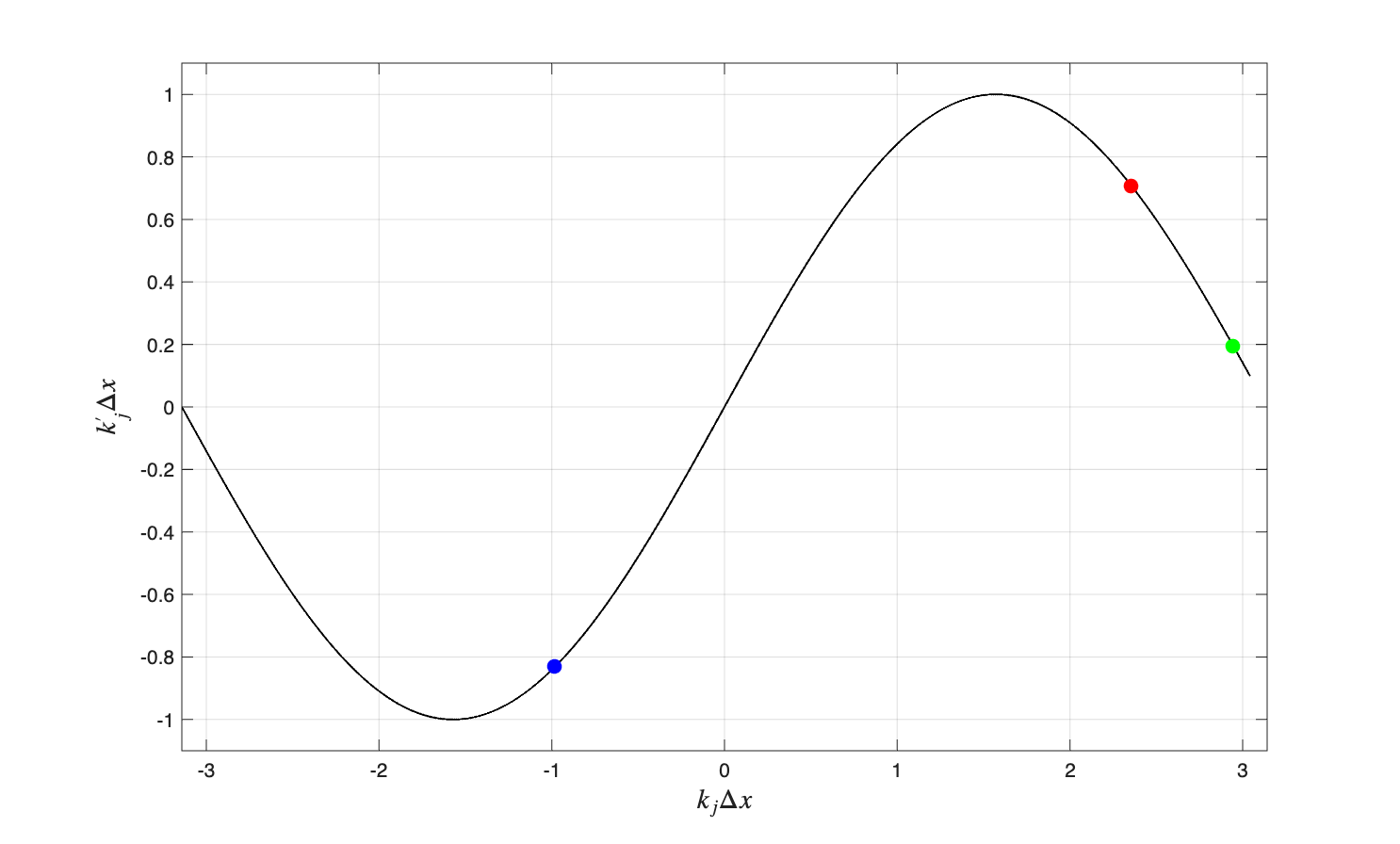
Thus, in the framework of DFT, a finite difference scheme is represented by a specific function \(k^{\prime }(k)\) which is typically periodic. Note that exact differentiation is given by \(k^{\prime } = k\) (not periodic).
So far we have discussed linear expressions and operators. Now we will examine Fourier transform of a nonlinear expression and its first derivative. Consider a finite Fourier expansion of a pointwise product \(w_m = q_m u_m\), as follows \[ w_m = q_m u_m = \sum _{j = -M/2}^{M/2-1} \sum _{l = -M/2}^{M/2-1} {\hat q}_j {\hat u}_l\, e^{\mathrm {i} (k_j+k_l) x_m} = \sum _{n=-M/2}^{M/2-1} {\hat w}_n e^{\mathrm {i} k_n x_m} \] with \(k_n = k_j + k_l\) and \({\hat w}_n\) are the Fourier coefficients associated with the product term \(w_m\). The double sum suggests there are products of Fourier modes with wavenumbers \(k_j+k_l\) that lie within the range of resolved wavenumbers but also modes whose wavenumbers are not in the resolved wavenumber range. As a result, these unresolved high-wavenumber modes are aliased to resolved lower wavenumber modes. This aliasing effect is simply a result of the quadratic nonlinearity. Since the wavenumber of an aliased mode differs from that of the unresolved one by \(2\pi M/L\), the Fourier coefficients of \(w_m\) may be written as [12] \begin {equation} {\hat w}_n = \sum _{j+l=n} {\hat q}_j {\hat u}_l + \sum _{j+l=n\pm M} {\hat q}_j {\hat u}_l\,, \quad n = -\frac {M}{2},\dots ,\frac {M}{2}-1 \label {eq:fcprod} \end {equation} Note that the second term on the right-hand side represents the aliasing error in the Fourier coefficient \({\hat w}_n\). However, the evaluation of the discrete product \(q_m u_m\) at grid points in physical space is not affected by aliasing and therefore remains exact. (If we would remove the second sum \(-\) an act that is called de-aliasing \(-\) and transform \({\hat w}_n\) back to physical space, we would not obtain the product \(w_m = q_m u_m\) at the grid vertices.)
Now let us look at what happens to the derivative of a product. Let \[ v_m = \frac {dq_m u_m}{dx} \] Applying DFT, one obtains \[ v_m = \sum _{j = -M/2}^{M/2-1} \sum _{l = -M/2}^{M/2-1} \mathrm {i} (k_j+k_l) {\hat q}_j {\hat u}_l \, e^{\mathrm {i} (k_j+k_l) x_m} = \sum _{n=-M/2}^{M/2-1} {\hat v}_n e^{\mathrm {i} k_n x_m} \] where \[ {\hat v}_n = \mathrm {i} k_n \sum _{j+l=n} {\hat q}_j {\hat u}_l + \mathrm {i} k_{n\pm M} \sum _{j+l=n\pm M} {\hat q}_j {\hat u}_l\,, \quad n = -\frac {M}{2},\dots ,\frac {M}{2}-1 \] We thus see that for the modes that contribute to the aliasing error, their Fourier coefficients are multiplied by the resolved (low) wavenumber of the aliased mode rather than its true (unresolved) wavenumber. This also applies to the spatial discretization of the derivative of the product, except that the Fourier coefficients are now multiplied by modified wavenumbers. Consider the following second order central differences \[ \frac {dq_mu_m}{dx} \approx \frac {q_{m+1} u_{m+1} - u_{m-1} u_{m-1}}{2\Delta x} \] By Fourier transforming this conservative expression, we obtain the following Fourier coefficients \begin {equation} \mathrm {i} k^{\prime }_n \sum _{j+l=n} {\hat q}_j {\hat u}_l + \mathrm {i} k^{\prime }_n \sum _{j+l=n\pm M} {\hat q}_j {\hat u}_l \label {eq:fcdivt} \end {equation} whereby noting that \(k^{\prime }_n = k^{\prime }(k_n)\) is periodic with period \(M\). Clearly, aliasing errors are altered by the truncation error of the above discretization. Depending on the function \(k^{\prime }(k_n)\), the effect of aliasing can either be small or large within the resolved wavenumber range.
Let us examine the modified wavenumbers of central differences as shown in Figure 7.1. We observe that they tend to reduce or even suppress the aliasing errors in the region near the ends of the positive wavenumber range \(k\Delta x \in [0,\pi ]\). However, the modified wavenumber of an aliased mode is typically intermediate and may thus slightly reduce aliasing errors. As an example, suppose that \(M = 64\) and consider the modes \(j = 24\) and \(l = 30\) (see red and green dots in Figure 7.1, respectively). These two modes are interacting and produce a third mode \(n =j+l = 54\) which will alias mode \(-10\). Since \(k^{\prime }(k_n)\) is periodic we have \(k^{\prime }(k_{54}) = k^{\prime }(k_{-10})\) (see blue dot). Referring to Figure 7.1, this results in a reduction of aliasing error by roughly 20%.
Now we consider the momentum advection in advective form as appeared in Eq. (\(\ref {eq:advt}\)). Thus, we evaluate the following expression at the grid point \(m\), \[ z_m = q_m\frac {du_m}{dx} \] The corresponding Fourier transform is given by \[ z_m = \sum _{j = -M/2}^{M/2-1} \sum _{l = -M/2}^{M/2-1} {\hat q}_j \, \mathrm {i} k_l \, {\hat u}_l \, e^{\mathrm {i} (k_j+k_l) x_m} = \sum _{n=-M/2}^{M/2-1} {\hat z}_n e^{\mathrm {i} k_n x_m} \] where \[ {\hat z}_n = \sum _{j+l=n} {\hat q}_j \, \mathrm {i} k_l \, {\hat u}_l + \sum _{j+l=n\pm M} {\hat q}_j \, \mathrm {i} k_l \, {\hat u}_l\,, \quad n = -\frac {M}{2},\dots ,\frac {M}{2}-1 \] Notice that the aliasing error is scaled by \(\mathrm {i} k_l\) due to the derivative \(du_m/dx\).
Next, we consider the following second order discretization of the advection operator \[ q_m\frac {u_{m+1} - u_{m-1}}{2\Delta x} \] The corresponding Fourier coefficients are thus given by \begin {equation} \sum _{j+l=n} {\hat q}_j \, \mathrm {i} k^{\prime }_l \, {\hat u}_l + \sum _{j+l=n\pm M} {\hat q}_j \, \mathrm {i} k^{\prime }_l \, {\hat u}_l \label {eq:fcadvt} \end {equation}
Let us revisit the previous example for this discretization. Mode \(l = 30\) has a relatively small modified wavenumber and according to Figure 7.1 the aliasing error is reduced by as much as 80% (see green dot). So we see in this specific example that the discretization of the momentum advection in advective form results in a smaller aliasing error than the discretization in divergence form.
So far we have not discussed the resolvable part of the Fourier coefficients of \(q_mu_m\), that is, the first convolution sum of Eq. (\(\ref {eq:fcprod}\)). We hereby assume that \(|j|, |l|, |n| \leq M/2\). We will analyze the effect of the discussed discretizations on this convolution sum. In the case of the discretization of the divergence operator \(v_m = dq_m u_m/dx\), this sum is multiplied by \(\mathrm {i} k^{\prime }_n\) (see Eq. (\(\ref {eq:fcdivt}\))), while it is multiplied by \(\mathrm {i} k^{\prime }_l\) when the advection term \(z_m = q_m\,du_m/dx\) is discretized (viz. Eq. (\(\ref {eq:fcadvt}\))). Let us restrict ourselves to positive wavenumbers, see Figure 7.2. (This is sufficient for the analysis here since both \(v_m\) and \(z_m\) are real.) Furthermore, we have \(k_n = k_j+k_l\).
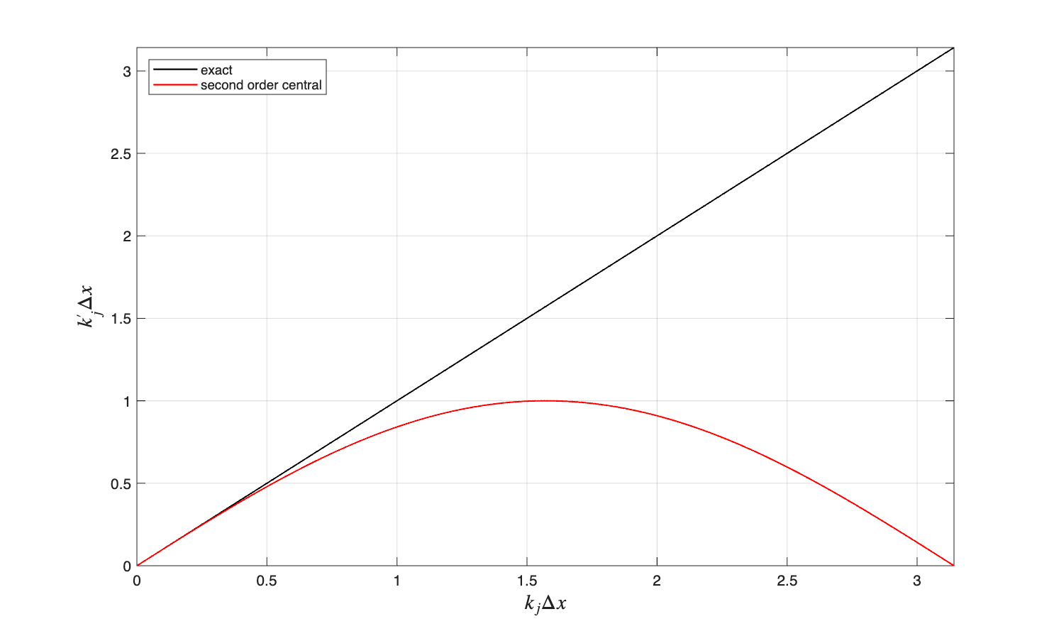
Since \(k_n > k_l\), the deviation from the exact differentiation is larger in the case of the discretization of the divergence operator than in the discretization of the advection operator. The effect of this is therefore a larger truncation error for the former than for the latter.
Based on the above we can therefore argue that the discretization of the momentum advection in advective form (\(\ref {eq:advt}\)) has generally a smaller discretization error (= truncation error + aliasing error) than the discretization in divergence form (\(\ref {eq:divt}\)). This conclusion is also supported by a number of examples presented in [112].
One final note. We chose the second order central difference scheme as an example above. However, in SWASH, we also apply the first order upwind scheme. Since this scheme is dissipative, the associated modified wavenumber consists of the real part and the imaginary part. The real part is equal to that of the second order central differences, see Figure 7.2. (The imaginary part represents a dissipation error.) In other words, the above analysis and conclusions also apply to the first order upwind scheme.
This chapter is yet empty. The following link is left here to give an idea of what the content of this material will look like: SWASH \(-\) sigmal layers.
This chapter is under preparation.
This chapter is under preparation.
We want to solve the following linear system of equations \begin {equation} A \, \vec {N} = \vec {b} \end {equation} where \(A\) is some non-symmetric penta-diagonal matrix, \(\vec {N}\) is the wave action vector to be solved and \(\vec {b}\) contains source terms and boundary values.
The basis for the SIP method (Stone, 1968; Ferziger and Perić, 1999) lies in the observation that an LU decomposition is an excellent general purpose solver, which unfortunately cannot take advantage of the sparseness of a matrix. Secondly, in an iterative method, if the matrix \(M = LU\) is a good approximation to the matrix \(A\), rapid convergence results. These observations lead to the idea of using an approximate LU factorization of \(A\) as the iteration matrix \(M\), i.e.: \begin {equation} M = L\,U = A + K \label {eq:lusip} \end {equation} where \(L\) and \(U\) are both sparse and \(K\) is small. For non-symmetric matrices the incomplete LU (ILU) factorisation gives such an decomposition but unfortunately converges rather slowly. In the ILU method one proceeds as in a standard LU decomposition. However, for every element of the original matrix \(A\) that is zero the corresponding elements in \(L\) or \(U\) is set to zero. This means that the product of \(LU\) will contain more nonzero diagonals than the original matrix \(A\). Therefore the matrix \(K\) must contain these extra diagonals as well if Eq. (\(\ref {eq:lusip}\)) is to hold.
Stone reasoned that if the equations approximate an elliptic partial differential equation the solution can be expected to be smooth. This means that the unknowns corresponding to the extra diagonals can be approximated by interpolation of the surrounding points. By allowing \(K\) to have more non zero entries on all seven diagonals and using the interpolation mentioned above the SIP method constructs an LU factorization with the property that for a given approximate solution \(\phi \) the product \(K\phi \approx 0\) and thus the iteration matrix \(M\) is close to \(A\) by relation (\(\ref {eq:lusip}\)).
To solve the system of equations the following iterations is performed, starting with an initial guess for the wave action vector \({\vec {N}}^0\) an iteration is performed solving: \begin {equation} U\,{\vec {N}}^{s+1} = L^{-1}\,K\,{\vec {N}}^s + L^{-1}\,\vec {b} \end {equation} Since the matrix \(U\) is upper triangular this equation is efficiently solved by back substitution. An essential property which makes the method feasible is that the matrix \(L\) is easily invertible. This iterative process is repeated \(s=0,1,2,...\) until convergence is reached.
This chapter is under preparation.
[1] A. Arakawa. Computational design for long-term numerical integration of the equations of fluid motion: Two-dimensional incompressible flow. Part I. J. Comput. Phys., 1:119–143, 1966.
[2] A. Arakawa and V. R. Lamb. Computational design of the basic dynamical processes of the UCLA general circulation model. Methods in Computational Physics: Advances in Research and Applications, 17:173–265, 1977.
[3] A. Arakawa and V. R. Lamb. A potential enstrophy and energy conserving scheme for the shallow water equations. Mon. Weather Rev., 109:18–36, 1981.
[4] R. Aris. Vectors, tensors and the basic equations of fluid mechanics. Prentice-Hall Inc., Englewood Cliffs, N.J., 1962.
[5] B. S. Baker, E. Grosse, and C. S. Rafferty. Nonobtuse triangulation of polygons. Discret. Comput. Geom., 3:147–168, 1988.
[6] R. Beltman. Mimetic discretizations of the incompressible Navier-Stokes equations for polyhedral meshes. Ph.D. thesis, Eindhoven University of Technology, 2020.
[7] G. A. Blaisdell, E. T. Spyropoulos, and J. H. Qin. The effect of the formulation of nonlinear terms on aliasing errors in spectral methods. Appl. Numer. Math., 21:207–219, 1996.
[8] P. B. Bochev and J. M. Hyman. Principles of mimetic discretizations of differential operators. In D. N. Arnold, P. B. Bochev, R. B. Lehoucq, R. A. Nicolaides, and M. Shashkov, editors, Compatible Spatial Discretizations. The IMA Volumes in Mathematics and its Applications, vol 142, pages 89–120, New York, NY, 2006. Springer.
[9] L. Bonaventura and T. Ringler. Analysis of discrete shallow-water models on geodesic delaunay grids with C-type staggering. Monthly Weather Review, pages 2351–2373, 2005.
[10] W. Boscheri, M. Dumbser, M. Ioriatti, I. Peshkov, and E. Romenski. A structure-preserving staggered semi-implicit finite volume scheme for continuum mechanics. J. Comput. Phys., 424, 2021. Article 109866.
[11] A. Bossavit. Whitney forms: a class of finite elements for three-dimensional computations in electromagnetism. In Science, Measurement and Technology, IEE Proceedings A, volume 135 (8), pages 493–500, 1988.
[12] C. Canuto, M. Y. Hussaini, A. Quarteroni, and T. A. Zang. Spectral Methods in Fluid Dynamics. Springer Verlag, New York, 1988.
[13] V. Casulli. Semi-implicit finite difference methods for the two-dimensional shallow water equations. J. Comput. Phys., 86:56–74, 1990.
[14] V. Casulli and R. A. Walters. An unstructured grid, three-dimensional model based on the shallow water equations. Int. J. Numer. Meth. Fluids, 32:331–348, 2000.
[15] V. Casulli and P. Zanolli. Semi-implicit numerical modeling of nonhydrostatic free-surface flows for environmental problems. Math. Comput. Modell., 36:1131–1149, 2002.
[16] J. C. Cavendish, C. A. Hall, and T. A. Porsching. A complementary volume approach for modeling three-dimensional Navier-Stokes equations using dual Delaunay/Voronoi tessellations. International Journal of Numerical Methods for Heat and Fluid Flow, 4:329–345, 1994.
[17] F. K. Chow and P. Moin. A further study of numerical errors in large-eddy simulations. J. Comput. Phys., 184:366–380, 2003.
[18] G. Coppola, F. Capuano, and L. de Luca. Discrete energy-conservation properties in the numerical simulation of the Navier-Stokes equations. Appl. Mech. Rev., 71:010803–1–19, 2019.
[19] C. J. Cotter and J. Shipton. Mixed finite elements for numerical weather prediction. J. Comput. Phys., 231:7076–7091, 2012.
[20] C. J. Cotter and J. Thuburn. A finite element exterior calculus framework for the rotating shallow-water equations. J. Comput. Phys., 257:1506–1526, 2014.
[21] Keenan Crane. Discrete differential geometry: An applied introduction. https://www.cs.cmu.edu/~kmcrane/Projects/DDG/paper.pdf, 2023. [Online; accessed 26 Sept 2023].
[22] P. J. Dellar. Common Hamiltonian structure of the shallow water equations with horizontal temperature gradients and magnetic fields. Phys. Fluids, 15:292–297, 2003.
[23] M. Desbrun, A. N. Hirani, M. Leok, and J. E. Marsden. Discrete exterior calculus. arXiv:math/0508341v2 [math.DG], pages 1–53, 2005.
[24] M. Desbrun, E. Kanso, and Y. Tang. Discrete differential forms for computational modeling. In A. I. Bobenko, P. Schröder, J. M. Sullivan, and G. M. Ziegler, editors, Discrete Differential Geometry, volume 38, pages 287–323. Birkhäuser Verlag, Basel, Switzerland, 2008.
[25] F. Ducros, F. Laporte, T. Souleres, V. Guinot, P. Moinat, and B. Caruelle. High-order fluxes for conservative skew-symmetric-like schemes in structured meshes: application to compressible flows. J. Comput. Phys., 161:114–139, 2000.
[26] F. N. Felten and T. S. Lund. Kinetic energy conservation issues associated with the collocated mesh scheme for incompressible flow. J. Comput. Phys., 215:465–484, 2006.
[27] O. B. Fringer, M. Gerritsen, and R. L. Street. An unstructured-grid, finite-volume, nonhydrostatic, parallel coastal ocean simulator. Ocean Modell., 14:139–173, 2006.
[28] M. Griebel, C. Rieger, and A. Schier. Upwind schemes for scalar advection-dominated problems in the discrete exterior calculus. In D. Bothe and A. Reusken, editors, Transport Processes at Fluidic Interfaces, pages 145–175. Springer International Publishing, 2017.
[29] C. A. Hall, J. C. Cavendish, and W. H. Frey. The dual variable method for solving fluid flow difference equations on Delaunay triangulations. Comput. Fluids, 20:145–164, 1991.
[30] F. E. Ham, F. S. Lien, and A. B. Strong. A fully conservative second-order finite difference scheme for incompressible flow on nonuniform grids. J. Comput. Phys., 177:117–133, 2002.
[31] W. Hansen. Theorie zur errechnung des wasserstandes und der strömungen in randmeeren nebst anwendungen. Tellus, 8:287–300, 1956.
[32] A. Hatcher. Algebraic Topology. Cambridge University Press, Cambridge, 2001.
[33] M. Herzfeld, D. Engwirda, and F. Rizwi. A coastal unstructured model using Voronoi meshes and C-grid staggering. Ocean Modell., 148, 2020. Article 101599.
[34] J. E. Hicken, F. E. Ham, J. Militzer, and M. Koksal. A shift transformation for fully conservative methods: turbulence simulation on complex, unstructured grids. J. Comput. Phys., 208:704–734, 2005.
[35] A. N. Hirani. Discrete Exterior Calculus. Ph.D. thesis, California Institute of Technology, Pasadena, California, USA, 2003.
[36] A. N. Hirani, K. B. Nakshatrala, and J. H. Chaudhry. Numerical method for Darcy flow derived using discrete exterior calculus. Int. J. Comput. Meth. Engng. Sci. Mech., 16:151–169, 2015.
[37] K. Horiuti. Comparison of conservative and rotational forms in large eddy simulation of turbulent channel flow. J. Comput. Phys., 71:343–370, 1987.
[38] J. M. Hyman and M. Shashkov. Natural discretizations for the divergence, gradient, and curl on logically rectangular grids. Computers Math. Applic., 33:81–104, 1997.
[39] A. Jameson, W. Schmidt, and E. Turkel. Numerical solution of the Euler equations by finite volume methods using Runge-Kutta time-stepping schemes. In AIAA 14th Fluid and Plasma Dynamic Conference, pages 1981–1259, Palo Alto, CA, 1981.
[40] C. A. Kennedy and A. Gruber. Reduced aliasing formulations of the convective terms within the Navier-Stokes equations for a compressible fluid. J. Comput. Phys., 227:1676–1700, 2008.
[41] H. W. J. Kernkamp, A. van Dam, G. S. Stelling, and E. D. de Goede. Efficient scheme for the shallow water equations on unstructured grids with application to the Continental Shelf. Ocean Dyn., 61:1175–1188, 2011.
[42] O. Kleptsova, J. D. Pietrzak, and G. S. Stelling. On a momentum conservative \(z\)-layer unstructured c-grid ocean model with flooding. Ocean Modell., 54-55:18–36, 2012.
[43] P. Korn and S. Danilov. Elementary dispersion analysis of some mimetic discretizations on triangular C-grids. J. Comput. Phys., 330:156–172, 2017.
[44] P. Korn and L. Linardakis. A conservative discretization of the shallow-water equations on triangular grids. J. Comput. Phys., 375:871–900, 2018.
[45] S. C. Kramer and G. S. Stelling. A conservative unstructured scheme for rapidly varied flows. Int. J. Numer. Meth. Fluids, 58:183–212, 2008.
[46] A. G. Kravchenko and P. Moin. On the effect of numerical errors in large eddy simulatons of turbulent flows. J. Comput. Phys., 131:310–322, 1997.
[47] J. Kreeft and M. Gerritsma. Mixed mimetic spectral element method for Stokes flow: a pointwise divergence-free solution. J. Comput. Phys., 240:284–309, 2013.
[48] J. J. Kreeft. Mimetic spectral element method \(-\) A discretization of geometry and physics. Ph.D. thesis, Delft University of Technology, 2013.
[49] J. J. Leendertse. Aspects of a computational model for long-period water-wave propagation. Ph.D. thesis, RM 5294-PR, Rand Corporation, Santa Monica, USA, 1967.
[50] D. Y. LeRoux, V. Rostand, and B. Pouliot. Analysis of numerically induced oscillations in 2D finite-element shallow-water models. Part I: inertia-gravity waves. SIAM J. Sci. Comput., 29:331–360, 2007.
[51] R. J. LeVeque. Finite Volume Methods for Hyperbolic Problems. Cambridge University Press, Cambridge, 2004.
[52] D. K. Lilly. On the computational stability of numerical solutions of time-dependent non-linear geophysical fluid dynamics problems. Mon. Weather Rev., 93:11–26, 1965.
[53] K. Lipnikov, G. Manzini, and M. Shashkov. Mimetic finite difference method. J. Comput. Phys., 257:1163–1227, 2014.
[54] T. A. Manteuffel and A. B. White Jr. The numerical solution of second-order boundary value problems on nonuniform meshes. Math. Comp., 47:511–535, 1986.
[55] C. Mattiussi. An analysis of finite volume, finite element, and finite difference methods using some concepts from algebraic topology. J. Comput. Phys., 133:289–309, 1997.
[56] C. Mattiussi. A reference discretization strategy for the numerical solution of physical field problems. Advances in Imaging and Electron Physics, 121:143–279, 2002.
[57] M. S. Mohamed, A. N. Hirani, and R. Samtaney. Comparison of discrete Hodge star operators for surfaces. Computer-Aided Design, 78:118–125, 2016.
[58] M. S. Mohamed, A. N. Hirani, and R. Samtaney. Discrete exterior calculus discretization of incompressible Navier-Stokes equations over surface simplicial meshes. J. Comput. Phys., 312:175–191, 2016.
[59] M. S. Mohamed, A. N. Hirani, and R. Samtaney. Numerical convergence of discrete exterior calculus on arbitrary surface meshes. Int. J. Comput. Meth. Engng. Sci. Mech., 19:194–206, 2018.
[60] Y. Morinishi, T. S. Lund, O. V. Vasilyev, and P. Moin. Fully conservative higher order finite difference schemes for incompressible flow. J. Comput. Phys., 143:90–124, 1998.
[61] P. J. Morrison. Poisson brackets for fluids and plasmas. In M. Tabor and Y. M. Treve, editors, Mathematical Methods in Hydrodynamics and Integrability in Dynamical Systems, pages 13–46, 1982. AIP Conf. Proc., no. 88.
[62] P. Mullen, A. McKenzie, D. Pavlov, L. Durant, Y. Tong, E. Kanso, J. E. Marsden, and M. Desbrun. Discrete Lie advection of differential forms. Found. Comput. Math., 11:131–149, 2011.
[63] J. R. Munkres. Elements of Algebraic Topology. Addison-Wesley Publishing Company, California, USA, 1984.
[64] T. Needham. Visual Differential Geometry and Forms. Princeton University Press, 2021.
[65] R. A. Nicolaides. Flow discretization by complementary volume techniques. In Proc. 9th AIAA Computational Fluid Dynamics Conference, pages 464–470, 1989. AIAA Paper 89-1978.
[66] R. A. Nicolaides. Direct discretization of planar div-curl problems. SIAM J. Numer. Anal., 29:32–56, 1992.
[67] R. A. Nicolaides. The covolume approach to computing incompressible flow. In M. D. Gunzburger and R. A. Nicolaides, editors, Incompressible Computational Fluid Dynamics, page 295, Cambridge, UK, 1993. Cambridge Univ. Press.
[68] R. A. Nicolaides. Three dimensional covolume algorithms for viscous flows. In M. Y. Hussaini, A. Kumar, and M. D. Salas, editors, Algorithmic Trends in Computational Fluid Dynamics, pages 397–414, New York, NY, 1993. Springer.
[69] A. Palha and M. Gerritsma. A mass, energy, enstrophy and vorticity conserving (MEEVC) mimetic spectral element discretization for the 2D incompressible Navier-Stokes equations. J. Comput. Phys., 328:200–220, 2017.
[70] N. Park, J. Y. Yoo, and H. Choi. Discretization errors in large eddy simulation: on the suitability of centered and upwind-biased compact difference schemes. J. Comput. Phys., 198:580–616, 2004.
[71] P. S. Peixoto and S. R. M. Barros. On vector field reconstructions for semi-Lagrangian transport methods on geodesic staggered grids. J. Comput. Phys., 273:185–211, 2014.
[72] B. Perot. Conservation properties of unstructured staggered mesh schemes. J. Comput. Phys., 159:58–89, 2000.
[73] B. Perot and R. Nallapati. A moving unstructured staggered mesh method for the simulation of incompressible free-surface flows. J. Comput. Phys., 184:192–214, 2003.
[74] J. B. Perot. Discrete conservation properties of unstructured mesh schemes. Annu. Rev. Fluid Mech., 43:299–318, 2011.
[75] J. B. Perot and V. Subramanian. Discrete calculus methods for diffusion. J. Comput. Phys., 224:59–81, 2007.
[76] J. B. Perot, D. Vidovic, and P. Wesseling. Mimetic reconstruction of vectors. In D. N. Arnold, P. B. Bochev, R. B. Lehoucq, R. A. Nicolaides, and M. Shashkov, editors, Compatible Spatial Discretizations. The IMA Volumes in Mathematics and its Applications, vol 142., pages 173–188, New York, NY, 2006. Springer.
[77] N. A. Phillips. An example of non-linear computational instability. In B. Bolin, editor, The Atmosphere and the Sea in Motion, pages 501–504, New York, 1959. Rockefeller Institute Press.
[78] S. A. Piacsek and G. P. Williams. Conservative properties of convection difference schemes. J. Comput. Phys., 6:392–405, 1970.
[79] T. Ringler, J. Thuburn, J. Klemp, and W. Skamarock. A unified approach to energy conservation and potential vorticity dynamics on arbitrarily structured C-grids. J. Comput. Phys., 229:3065–3090, 2010.
[80] M. Shashkov, B. Swartz, and B. Wendroff. Local reconstruction of a vector field from its normal components on the faces of grid cells. J. Comput. Phys., 139:406–409, 1998.
[81] T. G. Shepherd. Symmetries, conservation laws, and Hamiltonian structure in geophysical fluid dynamics. Advances in Geophysics, 32:287–338, 1990.
[82] A. Staniforth and J. Thuburn. Horizontal grids for global weather and climate prediction models: a review. Q. J. R. Meteorol. Soc., 138:1–26, 2012.
[83] P. K. Stansby. Semi-implicit finite volume shallow-water flow and solute transport solver with \(k\)-\(\varepsilon \) turbulence model. Int. J. Numer. Meth. Fluids, 25:285–313, 1997.
[84] S. Steinberg. The accuracy of numerical models for continuum problems. In H. Bulgak and C. Zenger, editors, Error Control and Adaptivity in Scientific Computing, pages 299–323, Dordrecht, The Netherlands, 1999. Springer.
[85] G. S. Stelling. On the construction of computational methods for shallow water flow problems. Ph.D. thesis, Rijkswaterstaat communications no. 35, 1984.
[86] G. S. Stelling and S. P. A. Duinmeijer. A staggered conservative scheme for every Froude number in rapidly varied shallow water flows. Int. J. Numer. Meth. Fluids, 43:1329–1354, 2003.
[87] G. S. Stelling and M. Zijlema. An accurate and efficient finite difference algorithm for non-hydrostatic free-surface flow with application to wave propagation. Int. J. Numer. Meth. Fluids, 43:1–23, 2003.
[88] G.S. Stelling and M. Zijlema. Numerical modeling of wave propagation, breaking and run-up on a beach. In B. Koren and C. Vuik, editors, Advanced computational methods in science and engineering, volume 71, pages 373–401, Springer, Heidelberg, 2010. Lecture Notes in Computational Science and Engineering.
[89] B. Strand. Summation by parts for finite difference approximations for \(d/dx\). J. Comput. Phys., 110:47–67, 1994.
[90] G. R. Stuhne and W. R. Peltier. A robust unstructured grid discretization for 3-dimensional hydrostatic flows in spherical geometry: A new numerical structure for ocean general circulation modeling. J. Comput. Phys., 213:704–729, 2006.
[91] J. Thuburn. Numerical wave propagation on the hexagonal C-grid. J. Comput. Phys., 227:5836–5858, 2008.
[92] J. Thuburn and C. J. Cotter. A framework for mimetic discretization of the rotating shallow-water equations on arbitrary polygonal grids. SIAM J. Sci. Comput., 34:B203–B225, 2012.
[93] J. Thuburn, T. Ringler, J. Klemp, and W. Skamarock. Numerical representation of geostrophic modes on arbitrarily structured C-grids. J. Comput. Phys., 228:8321–8335, 2009.
[94] E. Tonti. Why starting from differential equations for computational physics? J. Comput. Phys., 257:1260–1290, 2014.
[95] F. X. Trias, O. Lehmkuhl, A. Oliva, C. D. Perez-Segarra, and R. W. C. P. Verstappen. Symmetry-preserving discretization of Navier-Stokes equations on collocated unstructured grids. J. Comput. Phys., 258:246–267, 2014.
[96] E. Turkel. Accuracy of schemes with nonuniform meshes for compressible fluid flows. Appl. Numer. Math., 2:529–550, 1986.
[97] P. van Beek, R.R.P. van Nooyen, and P. Wesseling. Accurate discretization of gradients on non-uniform curvilinear staggered grids. J. Comput. Phys., 117:364–367, 1995.
[98] B. van’t Hof and A. E. P. Veldman. Mass, momentum and energy conserving (MaMEC) discretizations on general grids for the compressible euler and shallow water equations. J. Comput. Phys., 231:4723–4744, 2012.
[99] A. E. P. Veldman and K.-W. Lam. Symmetry-preserving upwind discretization of convection on non-uniform grids. Appl. Numer. Math., 58:1881–1891, 2008.
[100] A. E. P. Veldman and K. Rinzema. Playing with nonuniform grids. J. Engng. Math., 26:119–130, 1992.
[101] R. W. C. P. Verstappen and A. E. P. Veldman. Spectro-consistent discretization of Navier-Stokes: a challenge to RANS and LES. J. Engng. Math., 34:163–179, 1998.
[102] R. W. C. P. Verstappen and A. E. P. Veldman. Symmetry-preserving discretization of turbulent flow. J. Comput. Phys., 187:343–368, 2003.
[103] D. Vidovic. Polynomial reconstruction of staggered unstructured vector fields. Theoret. Appl. Mech., 36:85–99, 2009.
[104] J. Von Neumann and R. D. Richtmyer. A method for the numerical calculation of hydrodynamic shocks. J. Appl. Phys., 21:232–237, 1950.
[105] B. Wendroff and A. B. White Jr. A supraconvergent scheme for nonlinear hyperbolic systems. Comput. Math. Appl., 18:761–767, 1989.
[106] P. Wesseling, A. Segal, J.J.I.M. van Kan, C.W. Oosterlee, and C.G.M. Kassels. Finite volume discretization of the incompressible Navier-Stokes equations in general coordinates on staggered grids. Comput. Fluid Dyn. J., 1:27–33, 1992.
[107] H. Whitney. Geometric integration theory. Princeton University Press, Princeton, 1957.
[108] H. C. Yee and P. K. Sweby. Dynamical approach study of spurious steady-state numerical solutions of nonlinear differential equations. II. Global asymptotic behavior of time discretizations. Int. J. Comput. Fluid Dyn., 4:219–283, 1995.
[109] H. C. Yee, P. K. Sweby, and D. F. Griffiths. Dynamical approach study of spurious steady-state numerical solutions of nonlinear differential equations. I. The dynamics of time discretization and its implications for algorithm development in computational fluid dynamics. J. Comput. Phys., 97:249–310, 1991.
[110] X. Zhang, D. Schmidt, and B. Perot. Accuracy and conservation properties of a three-dimensional unstructured staggered mesh scheme for fluid dynamics. J. Comput. Phys., 175:764–791, 2002.
[111] M. Zijlema. TRIWAQ - three-dimensional shallow water flow model. Version 1.1. Technical documentation RKZ-438, National Institute for Coastal and Marine Management, The Hague, The Netherlands, 1998. SIMONA 99-01.
[112] M. Zijlema. The role of the Rankine-Hugoniot relations in staggered finite difference schemes for the shallow water equations. Comput. Fluids, 192, 2019. Article 104274.
[113] M. Zijlema. Computation of free surface waves in coastal waters with SWASH on unstructured grids. Comput. Fluids, 213, 2020. Article 104751.
[114] M. Zijlema. On the efficiency of staggered C-grid discretization for the inviscid shallow water equations from the perspective of nonstandard calculus. Mathematics, 10:1387–, 2022.
[115] M. Zijlema, A. Segal, and P. Wesseling. Finite volume computation of incompressible turbulent flows in general co-ordinates on staggered grids. Int. J. Numer. Meth. Fluids, 20:621–640, 1995.
[116] M. Zijlema and G. S. Stelling. Further experiences with computing non-hydrostatic free-surface flows involving water waves. Int. J. Numer. Meth. Fluids, 48:169–197, 2005.
[117] M. Zijlema and G. S. Stelling. Efficient computation of surf zone waves using the nonlinear shallow water equations with non-hydrostatic pressure. Coast. Engng., 55:780–790, 2008.
[118] M. Zijlema, G. S. Stelling, and P. B. Smit. SWASH: an operational public domain code for simulating wave fields and rapidly varied flows in coastal waters. Coast. Engng., 58:992–1012, 2011.